SMA ASIC Data Calibration with MIR/IDL
|
(1) Open MIR/IDL
| |
|
(2) Read the data into MIR
This data is single receiver only and just 400MB so it can all be read into MIR.
View a summary of the data.
All Sources: 3c273 NGC3175 0750+125 NGC2339 1037-295 0854+201 titan target All Baselines: 1-3 1-4 1-5 1-6 1-7 1-8 3-4 3-5 3-6 3-7 3-8 4-5 4-6 4-7 4-8 5-6 5-7 5-8 6-7 6-8 7-8 All Recs: 230 All Bands: c1 s01 s02 s03 s04 s05 s06 s07 s08 s09 s10 s11 s12 s13 s14 s15 s16 s17 s18 s19 s20 s21 s22 s23 s24 All Sidebands : l u All Polarization states: hh vv hv vh All Integrations: 0-754 | |
|
(3) Flag pointing data
Pointing data will have an integration time < 10seconds. Use dat_filter to select just this data, then flag the selection.
Use the if loop to prevent all data being flagged in the event there is no pointing data.
Afterwards, re-select only the positive weighted (unflagged data).
| |
|
(4) Inspect the data visually
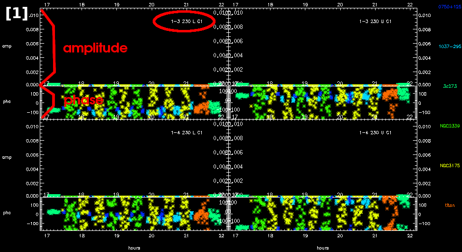
Plot the pseudo-continuum channel [1]. This is an average of the spectral channels for each point for both ampltude and phase.
Scroll through the plots by right-clicking. Use the middle-click to bring up a menu in the terminal. One option will be f for flag. Select f then left-click on an point to flag it [2]. When you flag a point interactively the scan number is reported in the terminal. Once you have finished flagging exit with a right-click. You will see outliers appearing at the same position across baselines and sidebands [2]. To avoid having to flag each one separately, use the interactive plotting to get the scan number, then select and flag it on all baselines.
Select just positive weighted data and re-plot.
As the scaling changes another outlier appears - scan number 7. This step may require a few iterations. Finally the data will look like [3].
|


|
|
(5) Apply the system temperature correction
View the system temperature. Check the points and profile for outliers.
Here the data all looks reasonable. The correction can be applied without further issue. See the SWARM page for examples of fixing problems with system temperature data
Then regenerate the continuum channel.
| 
|
|
(6) Check for spikes
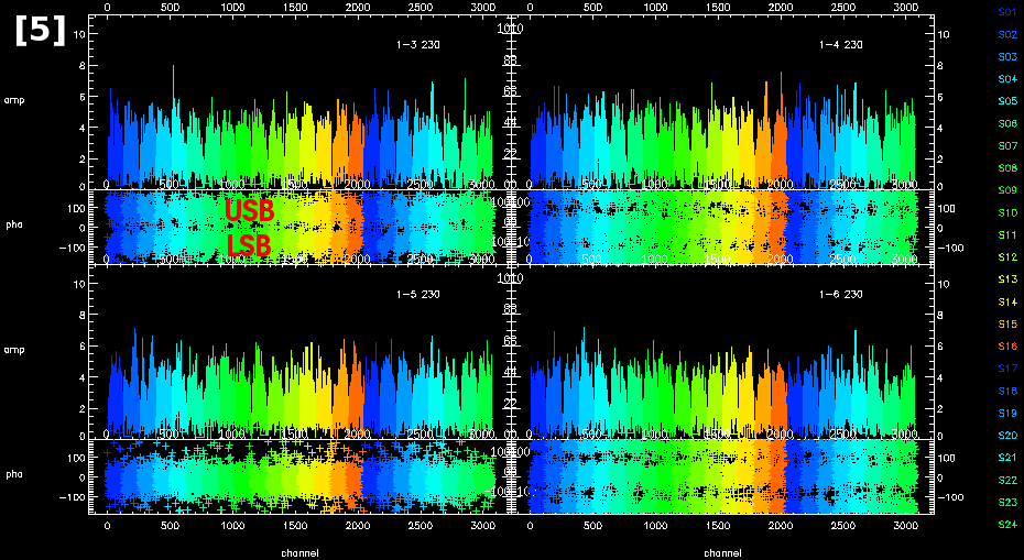
Inspect the frequency data for spikes. by default plot_spectra has x='channel' [5]. You can plot using x='fsky' for frequency, but should do so separately for each sideband as there is a large separation between them.
Right-click to scroll through the plots for each source. If you see a spike you will need to plot only the spectral window it lies in, in order to determine it's correct channel number for flagging. Although it's not very big we will flag the spike in spectral window s08.
Zooming in you can identify the channel number as 35. Then apply the fix.
Reselect all data.
By default, uti_chanfix replaces the value of the given channel with an average of the adjacent 3rd channel on each side. Set which channels will be used to produce the average with the option 'sample'. If a spike is a few channels wide for example, using sample=10 will use the 10th channel on either side for an average. The SWARM example uses the uti_checkspike task to automate this step. |

|
|
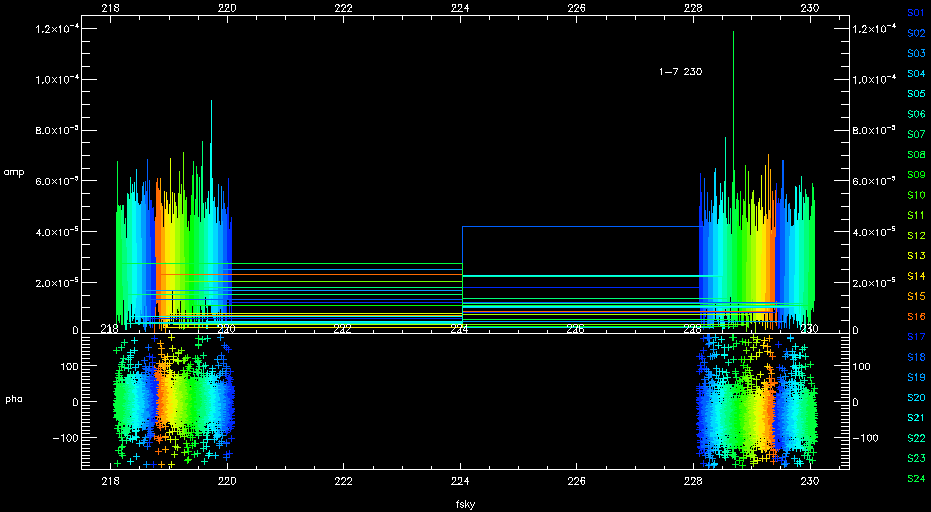
(7) Perform bandpass calibration
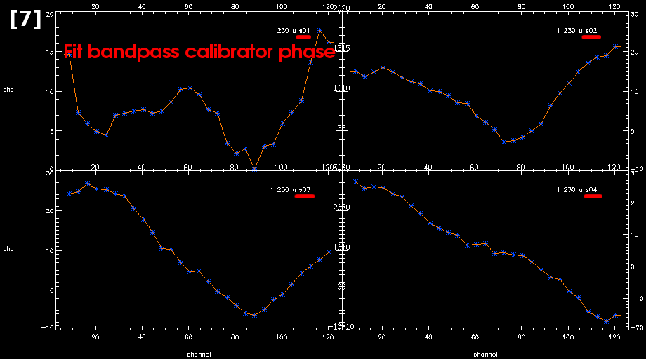
Apply the phase based bandpass first. Use the /preavg option which averages the selected number of channels into a single point.
 Check: Found a total of            6  different sources in the data set.
 Set which sources will be used as calibrators and set the calibrator fluxes
 The flux should be in Jy at the frequency of the observation
 These are the sources and their current passband codes
 name:  3c273              passband cal: NO
 name:  NGC3175            passband cal: NO
 name:  0750+125           passband cal: NO
 name:  NGC2339            passband cal: NO
 name:  1037-295           passband cal: NO
 name:  titan              passband cal: NO
 Enter source and new cal code. eg: 3C273 YES
 or hit Return if all the sources are correctly specified
  : 3c273 yes
At this stage there is the option to accept the sources it suggests or add/remove any. Usually the bandpass calibrator(s) is identified as such in the software (and listed as YES) but not always. Here 3c273 is added by typing 3c273 yes. Once it has generated a solution it will create a plot of the fits [7]. Right-click through the solutions for each baseline. After exiting the plot window it will prompt to accept or reject the solutions. If pass_cal fails reporting insufficient flux, try adding more sources to the list (if suitable ones are available), or increasing the 'preave' value to increase the signal-to-noise. NOTE: ASIC data may have a different resolution for each chunk. Be sure to perform bandpass calibration separately for each resolution. Now regenerate the continuum. Fixing the phases will slightly boost the average amplitudes for the next step.
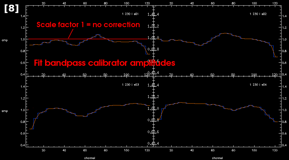
Next repeat the process in the same way for amplitude [8].
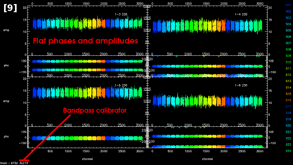
Check the success of the bandpass calibration by viewing the spectra for the bandpass calibrator. The phases and amplitudes look nice and flat [9].
|
|
|
(8) Save the data
Select all unflagged data, regenerate the continuum and save in MIR format. It is important to save the dataset before starting flux measurement as the phases will be irreversibly disrupted.
| |
|
(9) Flux measurement
It does not matter which order gain calibration and flux calibration occur. Select all the flux and gain calibrators.
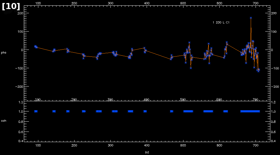
Apply the gain_cal in phase first with the /connect option to force the phases to zero for every scan [10]. The /non-point option takes into account the size of planets, on some baselines resolved planets may have a phase of ±180°.
Next run amplitude based gain_cal [11]. Here, only select the flux calibrator (usually a planet or moon). Using the /non-point option it will retrieve its flux.
    : all no
    : titan yes
Note: the task sma_flux_cal performs the same amplitude based gain calibration as above, but baseline rather than antenna based. Ideally, select quasar scans near the flux calibrator in time and/or elevation. The conditions (pointing, opacity, system) should be as similar as possible when scaling between the flux calibrator and gain calibrators. In this data, the quasar scans near the flux calibrator are below 35° elevation which isn't ideal. Now measure the calibrated flux with flux_measure. It will return either vector or scalar values for each source. Scalar values ignore phase noise, so the amplitudes are typically slightly higher.
|

|
|
(10) Gain calibration on the restored data
With known fluxes for the gain calibrators, restore the previously saved file and perform gain calibration.
Select just the science and the gain calibrator sources.
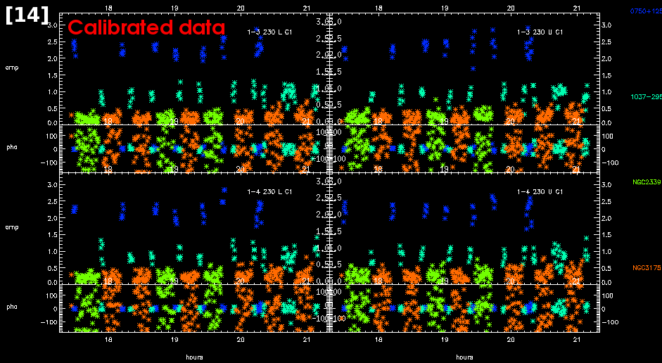
Apply the phase based gain_cal using smoothing and /preavg [12].
   : 0750+125 yes 2.3014
   : 1037-295 yes  0.8437
|

|
|
(10) Save the calibrated data
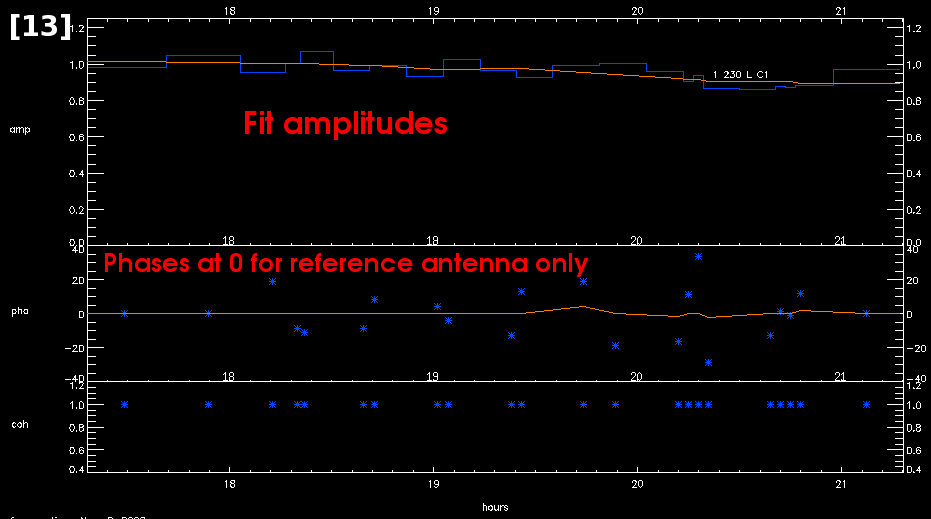
Have a final check of the calibrated dataset [14]. There remains some scatter in the calibrator amplitudes, but the phases are flat and overall the calibration looks good. This data was taken in very extended configuration which is generally worse than data taken in compact configuration.
Then save the data in MIR format.
Export continuum and spectral data to MIRIAD.
Save the data in uvfits format to be read by CASA.
|
 |