The graphic display tool smauvspec was developed based on the original Miriad routine uvspec. The task, smauvspec, plots averaged spectra of a visibility dataset for all the SMA spectral chunks in one sideband with a color coded for each spectral chunk data or for specific spectral windows using the function select. Averaging can be made in both time and frequency along the x-axis.
smauvspec% inp
  Task:   smauvspec
  vis      = gc_rx1.lsb.tsys      % input name of the uv data
  stokes   = xx
  interval = 3                    % 3 min in average
  axis     = chan,ampl            % plot amplitude vs channel;
             or (chan, phas)        plot phase vs channel.
  device   = /xs                  % pgplot device: x-window
  nxy      = 7,4                  % 7 by 4 panels on each page
                                    this plots a snapshot of all
                                    the spectral data per page
                                    for all 28 baselines.
  log      =
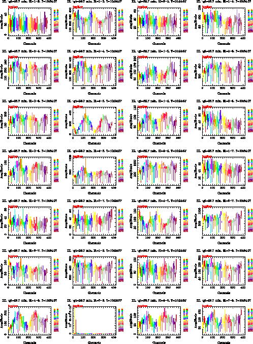
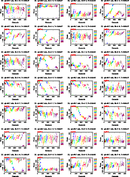
With smauvspec users can inspect the spectral data in various ways. The above example shows a way to quickly go through all the data and to see if there is any bad data that might contaminate the spectra. Fig.2.5 shows the 24 spectral chunks (coded color) of Jupiter on 28 baselines. It is obvious that the baseline 5-8 has a problem. This problem is present on all sources during the observation. It turns out that the problem was due to a bad correlator chip of the first block of spectral chunks (s1,s2,s3,s4) on this particular baseline. Note that the SMA spectral band id (a number preceded with letter s) is coded in the SMA archival data but is not used in Miriad. The phase plot (Fig.2.6) also shows the problem.
 |
 |
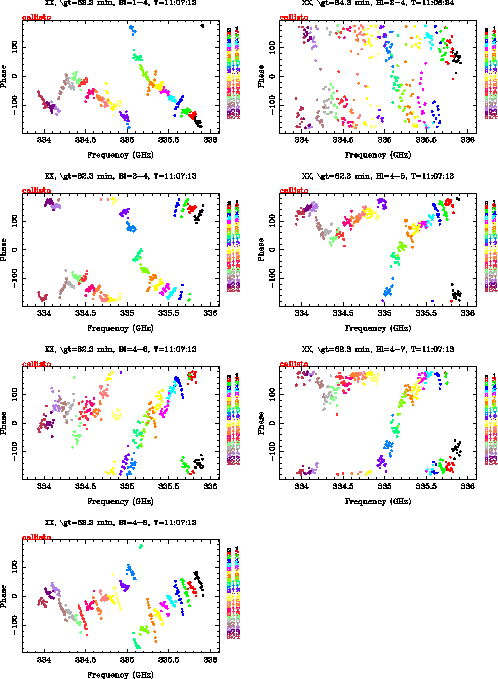
Now, we take a particular antenna (4) to have a close look at its phase. The input parameters of smauvspec below demonstrate an example to look at the phase on the antenna (4) from snapshot spectra of Callisto. A phase delay is clearly seen on the baselines related to antenna 4 (see Fig.2.7).
The Miriad functions select and line give a variety of options to select data. Please read Section 2.3 - Utility Functions in this Guide or the original Miriad User's guide (both BIMA and ATNF versions) for the details.
smauvspec% inp
  Task:   smauvspec
  vis      = gc_rx1.lsb.tsys
  select   = source(cal*),ant(4)
  stokes   = xx
  interval = 30
  axis     = freq,phas
  device   = /xs
  nxy      = 2,1
 |