ˇˇ
Cloud Optical Thickness and Radius Retrieval
![]()
This document describes the detailed procedures to perform cloud optical thickness and radius retrieval using GOES data. This image is a GOES-8 image taken in the Pacific Ocean in West Coast of America [30.5-41.5N, 151.1-116.9W], at local noon on July 15, 1998. Four channels’ data are provided except water vapor channel 3. The shortwave (SW) and the longwave (LW) part of channel 2 are provided separately. The provided data are similar to AVHRR except that it does not have the near-infrared channel. Four tests are applied to detect cloud-contaminated pixels and differentiate water clouds and ice clouds.
1. Cloud Detection and Classification
2. Results and Discussions for Cloud Detection
The results for each test are shown in Figure 1. We can see that the visible threshold test is very effective in this case, that detects almost all the cloud-contaminated pixels. The infrared gross cloud check can only detect those clouds with lower temperature. It cannot well detect those marine stratus clouds, since they have close temperature to ocean surface temperature. Actually, from the histogram of channel 5, only one peak is found, consisting of both clear-sky pixels and stratus. The ice clouds are those brightest clouds, which can be seen from the visible image. The mixed phased clouds are located in the bottom left corner and neighboring to ice clouds.
|
|
Figure 2. Classfied image for the image in Figure 1. |
|
| Figure 1. Results after each test of cloud detection. |
According to the results of cloud detection, the image features are fallen into four categories: ocean clear sky, water clouds, mixed-phased clouds and ice clouds. The color-coded classification image is shown in Figure 2. The mean value and standard deviation of each class for each channel, and the area coverage for each class are listed in Table 1.
Table 1. Mean and standard deviation for each class, and Area Coverage
Classes |
Area Coverage (Percentage) |
Channels(unit) |
Mean |
Standard Deviation |
| Ocean Clear Sky |
13995.3 km2 (34.2%) |
1 (%) |
5.88 |
1.92 |
2 % |
0.95 |
1.6 |
||
2 (K) |
289.19 |
3.97 |
||
4 (K) |
287.70 |
3.56 |
||
5 (K) |
287.55 |
3.41 |
||
| Water Clouds |
23939.4 km2 (58.5%) |
1 (%) |
21.86 |
7.65 |
2 (% ) |
4.61 |
3.39 |
||
2 (K) |
292.87 |
5.17 |
||
4 (K) |
285.49 |
2.29 |
||
5 (K) |
285.77 |
2.44 |
||
| Mixed-phased Clouds |
2209.8 km2 (5.4%) |
1 (%) |
34.70 |
10.7 |
2 (% ) |
2.93 |
1.95 |
||
2 (K) |
273.27 |
7.69 |
||
4 (K) |
260.57 |
9.84 |
||
5 (K) |
259.57 |
9.48 |
||
| Ice Clouds |
777.5 km2 (1.9%) |
1 (%) |
47.00 |
5.40 |
2 (% ) |
1.90 |
0.53 |
||
2 (K) |
258.35 |
4.40 |
||
4 (K) |
237.50 |
5.25 |
||
5 (K) |
236.88 |
5.98 |
The results obtained above are reasonable compared to what we have learned in Remote Sensing I and II. The ocean clear sky reflectance is about 6% at channel 1, and only 0.95% at channel 2. Water clouds (marine stratus or fog) have an average reflectance of 21% at channel 1. This low reflectance of water clouds is due to that the water clouds in the middle of the image are partly and thin clouds. Note that the channel 4 and channel 5 temperature for water clouds are only 2 degree smaller than those of ocean clear sky, that’s’ why the infrared gross cloud check is not effective in detecting low clouds such as marine stratus and fog. The channel 2 temperature is even 3.5 K greater than the clear sky value. It might be due to some errors when deriving the channel 2 longwave part of radiation from channel 4 radiance. The reflectance at channel 2 for water is about 4.6%. From water clouds to mixed-phased clouds to ice clouds, channel 2, 3, 4 temperature decreases and the ch1 reflectance increases. However, channel 2 reflectance decreases because ice has stronger absorption than liquid water.
If increase (decrease) the temperature threshold by 5% in Celsius (0.32 K), the clear pixels coverage decrease (increase) only by 0.15%, and vice versa for water clouds coverage. This small effect is negligible and is due to that the dynamic visible reflectance test is more effective in detecting clouds in this case. The effects on mean and standard deviation is negligible at all. Even perturb by 3 K, the coverage for clear and water clouds is still within 1.5%, the effects on mean and standard deviation are negligible. If the visible threshold 10.5% increases (decreases) by absolute 5%, i.e. to 15%(5%), it will largely affect the area coverage for clear and water clouds. 13% more (less) pixels are classified as clear and 13% less (more) are classified as water clouds, clear sky reflectance at channel 1 increases (decreases) by 2%, the channel 1 reflectance for water clouds increase by 3%. The effects on mean ch2, ch4, ch5 temperature are small since the temperature difference between water clouds and clear sky is small. If the visible threshold 10.5% increases (decreases) by relatively 5%, i.e. to 11%(10%), the percentage of area coverage for clear sky increases (decreases) by 1%, the channel 1 reflectance increases to 6.0% (decreases to 5.6%). Therefore, detecting clouds using thresholds depend on the quality of selected threshold and their relative contribution in detecting clouds.
3. Optical Thickness and Radius Retrieval
3.1 Model set-up in SBDART CODE
The wavelength range for channel 1 is 0.52 to 0.72 m m with interval of 0.005 m m. The wavelength range for channel 2 is 3.78 to 4.03 m m with interval of 0.025 m m. The response function is assumed as the same as VIRS, i.e. 27 for channel 1 and 28 for channel 2. The image is taken in Mid-latitude regions in July, so mid-latitude summer atmospheric profiles are assumed with a water vapor of 2.924 g/cm2. The surface albedo for channel 1 is assumed as 3.5% by subtracting about 2% from the mean ocean clear sky reflectance obtained in Table 1. The surface albedo for channel 4 is assumed as 0.4% by subtracting 0.5% from the mean value. The solar zenith angle in this image ranges from 9?to 26?, so a loop of 5 solar zenith angle (9?, 14?, 19?, 24?, 29?) is set. A loop of 7 value is set for optical depth (0, 2, 4, 8, 12, 18, 36) and effective particle size (2 m m , 4 m m, 6 m m, 8 m m,12 m m, 18 m m, 36 m m), respectively. The droplet size distribution for water clouds (Input of documentation of SBDART, cloud//c1/data/ats770/sbdart) is assumed as gamma distribution (Further discussion later). For each solar zenith angle, optical depth and particle size, I calculate the radiance at 10 relative azimuthal angles (from 60?to 150?every 10 degree) and 7 view zenith angles (57?, 62?, 67?, 72?, 77?, 82?, 88?).
3.2 Interpolation Procedure
Figure 3 shows the calculated bispectral reflectance plot as a function of solar zenith angle (top), view zenith angle (middle) and relative azimuthal angle (bottom). We can see that the solar zenith angle dependence is small due to a small solar zenith angle range in this image. The channel 1 reflectance is larger at 29?than at 9?. There is a stronger dependence of view zenith angle in the view zenith angle range of this image. Both channel 1 and channel 2 reflectance decrease with the increase of view zenith angle. The channel 1 and channel 2 beyond 82?is very small, using them to retrieve properties will lead to larger uncertainties. Therefore, cloudy pixels with view zenith angle larger than 77?(only 18 pixels) are not retrieved. The effects of azimuthal angle are very small. Since in this case, the bispectral reflectance plot is not so sensitive to solar zenith angle and azimuthal angle, so for an individual pixel, I retrieve cloud properties using look-up table closest to its solar zenith angle and azimuthal angle. As for view zenith angle, I retrieve two cloud properties at two view zenith angles around individual view zenith angle, and then use linear interpolation (as to cosine of view zenith angle) to get the cloud optical depth and particle radius.
After identifying look-up tables for an individual pixel, the procedure is as follows. Each constant optical depth line and constant effective particle size line on the bispectral plot are simulated by a three-order polynomial fitting (almost completely overlap with the data points), and so we can get a equation for each line. Given a pair of ch 1 and ch 2 reflectance of a pixel, we can find the grid where it lies on the bispectral plot according to the simulated equations. Draw a horizontal line from measurement point and get two points where it intersects with two constant optical depth lines. Then we can get the retrieved optical depth by using linear interpolation. The effective particle size can be retrieved as well by drawing vertical line. The cloud liquid water path is 2/3 of the product of optical depth and effective particle radius. If a measurement is located in the left side of iso-optical thickness line of 2, the cloud properties are not retrieved, since there would have very large uncertainty in the retrieved results. Only water clouds are retrieved.
|
|
| Figure 3. Reflectance as a function of optical thickness and particle radius for different viewing geometry. |
3.3 Results and discussions
Table 2. Statistics for derived Properties of Water Clouds
Profile |
Optical depth |
Effective Particle Size (µm) |
Cloud Liquid Water Path (g/m2) |
|||
Mean |
S. D. |
Mean |
S. D. |
Mean |
S. D. |
|
Mid-latitude Summer |
5.08 |
2.12 |
22.71 |
11.46 |
73.61 |
45.89 |
Tropical |
4.94 |
2.13 |
21.29 |
11.59 |
66.97 |
44.46 |
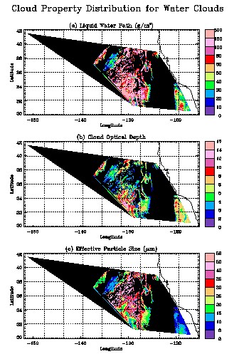
The histogram of optical depth, cloud droplet size and cloud liquid path is shown in Figure 4. The mean and standard deviation of optical depth, particle depth and cloud liquid water path are shown in Table 2. The effective particle size presents a three-mode distribution, at about 10, 17, and 35 m m, respectively, corresponding to different stages of cloud development. The optical depth peaks at about 5, indicating that most of the water clouds in this image are thin clouds or partly cloudy. The cloud liquid water path peaks at about 20-80 g/m2. The color-coded images of cloud water path, optical depth and droplet size are shown in Figure 5 (The horizontal line and vertical lines are for problem d about the transect line). The clouds in the top right corner have small particle size 6-15 m m, medium optical depth of 6-8 and liquid water path of 30-80 g/m2. The water clouds with largest optical depth labeled as A in Figure 6 also has larger optical particle size (greater than 20 m m) and larger cloud water path. These are thick stratus clouds. Some of the linear-formed clouds labeled as B has very large particle size greater than 35 m m, small optical depth as small as 3-4. These clouds are probably formed due to ship track. The region labeled as C is associated with very large particle size greater than 35 m m and small optical depth of 3-4. These are thin stratus clouds, drizzle could happen in these regions.
If the mid-latitude summer profiles is changed to tropical profiles, the main factor that affect the results is that there is more water vapor. The water vapor for tropical profile used in SBDART is 4.117 (g/m2). If containing more water vapor, the effect on visible channel 1 reflectance is negligible but the channel 3 reflectance will decrease due to water vapor absorption. By looking at the look-up table, if decrease the channel 2 reflectance (look-up table itself), we will get smaller particle size for the same measurements. The statistics including mean and standard deviation using tropical profiles is also provide in Table 2. The particle size decreases by 1.5 m m, the mean optical depth remains almost the same, and the cloud water path decreases by 7 g/m2.
|
|
| Figure 5. Color-coded image of cloud optical thickness, cloud optical path and effective particle size. | Figure 6. Geo-located image of cloud optical thickness, cloud optical path and effective particle size. |
Appendix: Derivation of Liquid Water Path
According to the definition of optical thickness t :
![]()
Where Qext is the extinction coefficiency, r is particle size, n(r) is particle size distribution, and z is the physical depth. For water clouds at visible channel, liquid water absorption is negligible, then the Qext can be assumed as 2. The vertically integrated liquid water path (LWP) can be expressed as:
Where r is density of water, and can be approximated as 1 .0 x 106 g/m3. Since from satellite remote sensing, only the properties of clouds in the upper part can be retrieved, to get the LWP for the whole vertically integrated clouds, we assume that the liquid water content in the lower part is the same as the upper part, and n(r,z) is independent of z, then:
According to equation (2), the LWP is dependent on droplet number concentration and physical depth. If the number droplet concentration is tripled, and the liquid water path is only doubled, then the physical depth must be decreased by 2/3 provided the above assumptions are right. Anyway, the effective particle radius doesn’t change. According to equation (3), the optical thickness will be doubled the same as LWP.
References
Saunders R. W., R. T. Kriebel, An improved method for detecting clear sky and cloudy radiances from AVHRR data, Int. J. Remote Sensing, 9(1), p123-150, 1988.
![]()
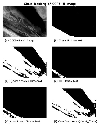
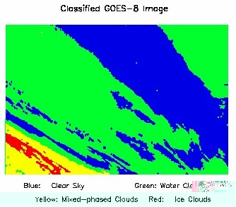
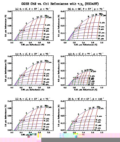
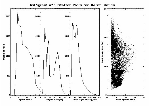 Figure 4. Histogram of
retrieved optical depth, cloud droplet size and cloud liquid path.
Figure 4. Histogram of
retrieved optical depth, cloud droplet size and cloud liquid path.