Applications of PETSc to open questions in planet formation theory
Ellen M. Price
Center for Astrophysics | Harvard & Smithsonian
PETSc '19, 7 June 2019
Hi, my name is Ellen Price, and I'm a rising fifth-year
graduate student at the Center for Astrophysics |
Harvard & Smithsonian, a collaboration between
Harvard University's astronomy department and the
Smithsonian Institution. Today, I'd like to
talk to you about how I've applied the PETSc software
to my research in the field of planet formation.
Before I get started, though, I'd like to thank the
conference organizers for inviting me and putting
together a terrific event.
Coauthors
Prof. Karin Öberg (Harvard)
Prof. Ilse Cleeves (UVa)
Prof. Leslie Rogers (UChicago)
Next, I'd like to thank my coauthors and advisors,
since none of the projects I will discuss today
would be possible without them. Prof. Öberg is
my primary advisor at Harvard, and we work closely
with Prof. Cleeves, now at the University of Virginia,
on the second project I'll talk about. The first
project is one that I work on with Prof. Rogers,
at University of Chicago, and using their
Research Computing Center for computation.
Outline of today's talk
Introduction to exoplanets
Project 1: SQUISHv2 and tidally distorted rocky planets
Introduction to planet formation
Project 2: Coupling accretion and chemistry in protoplanetary disks
Questions
Here, I'm just going to give you an idea of what's
coming up in this talk. First, I'd like to give some
background on exoplanets; I'll be assuming you know
little about the topic, so this should be a
comprehensive overview. Next, I'll talk
about a project that uses PETSc for exoplanet theory.
Then, I'll give an overview of planet formation,
which is a closely-related topic, and discuss a
second project in that field. Finally, I'll take any
questions and we can have some open discussion. If
you do have questions during the talk, I welcome you
to ask, especially if something I say is unclear.
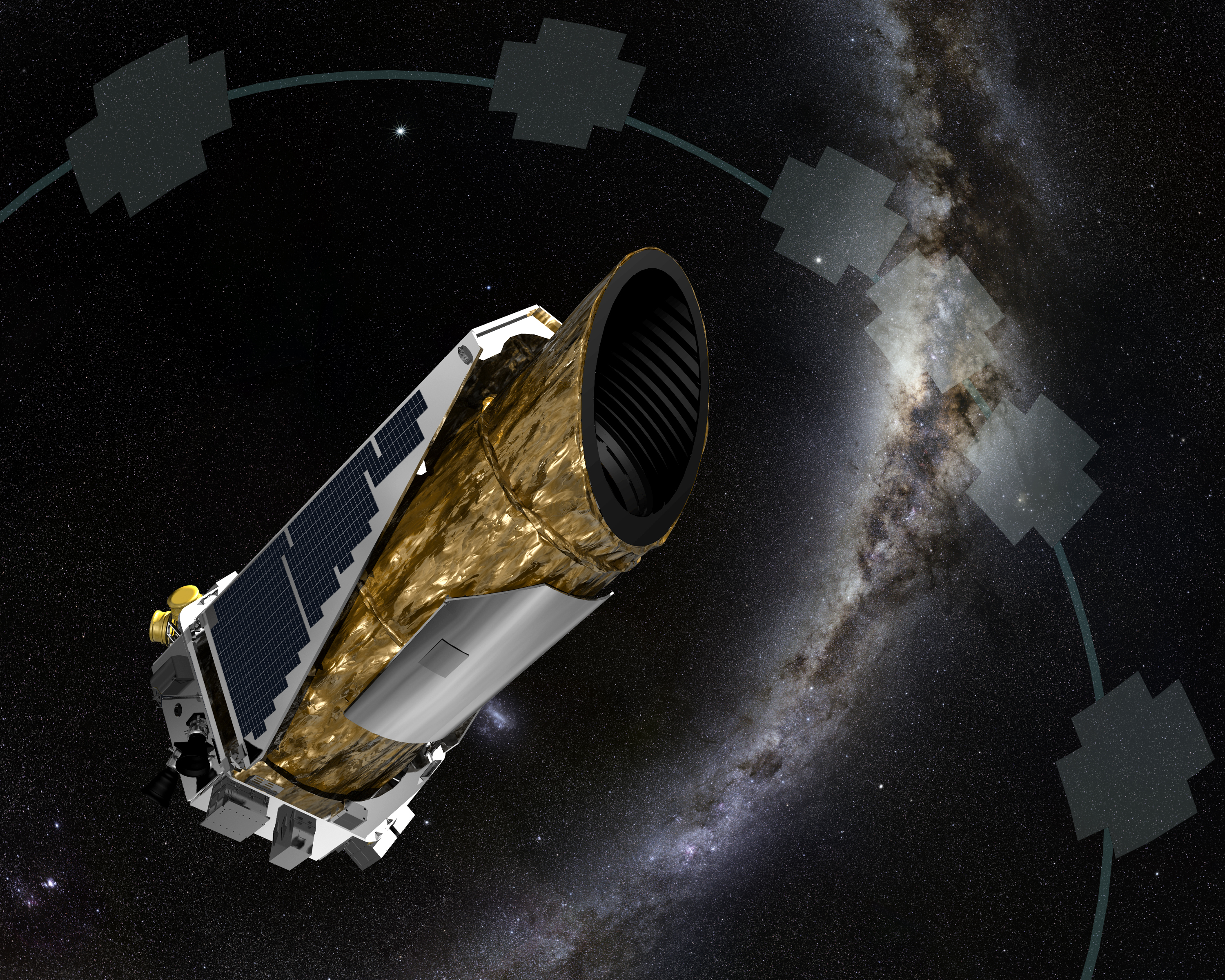
Exoplanets and their properties
Discovering planets
(source: nasa.gov)
In 2009, we launched the Kepler space telescope;
its mission was to identify planets in our galaxy but
outside the Solar System, which are called exoplanets,
including Earth-like planets. The spacecraft has since
experienced a critical failure in its reaction wheels
that caused the field of view to change, yet it is
still finding planets under the new mission name, K2.
The fields of view on this image are for the K2
mission, but they still give you an idea of what
Kepler saw during its original mission.
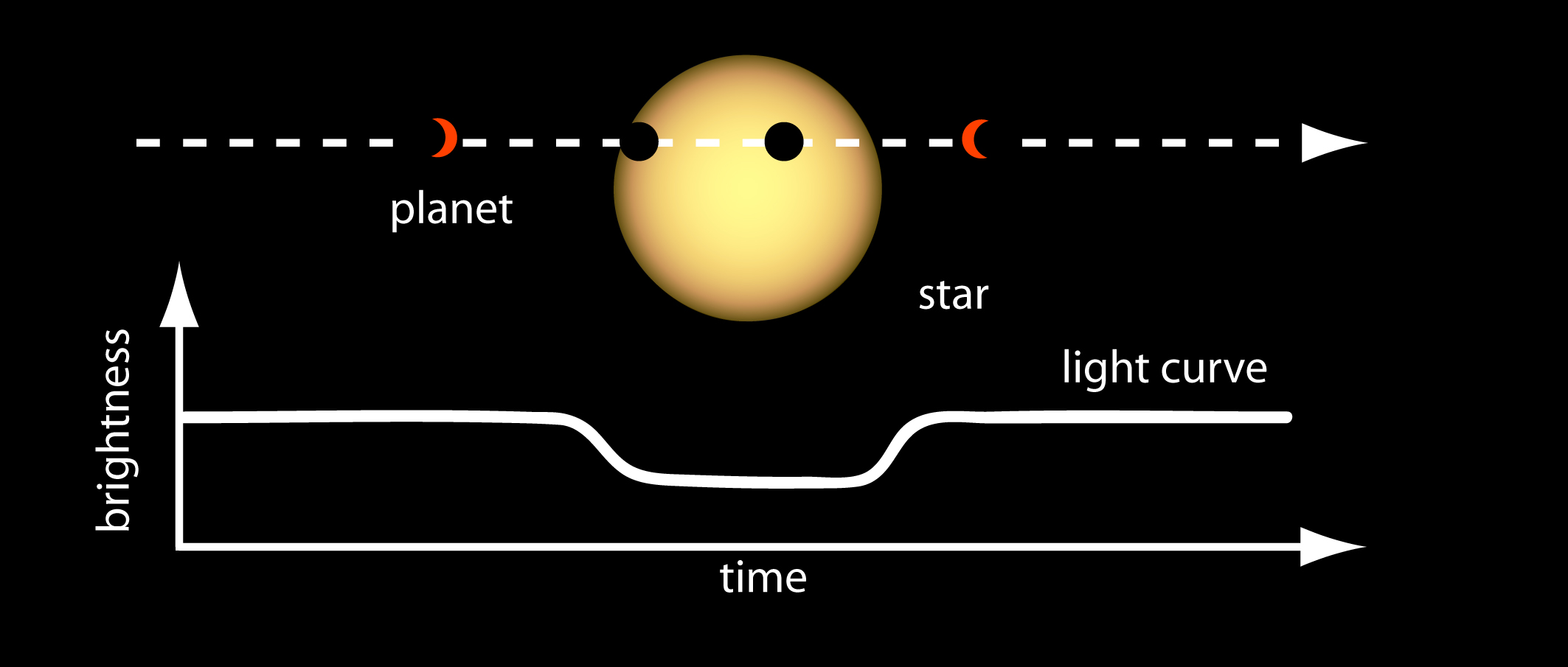
Detecting planets
(source: jpl.nasa.gov)
What do we mean when we say that Kepler is
able to detect exoplanets? Kepler uses the
transit method of detection, which involves measuring
the light from a star and watching for these
characteristic “dip” shapes that indicate
the presence of a planet, where the planet has blocked
some of the light from the star in a predictable way.
You can imagine that star spots will do the same
thing, however, which presents a significant challenge
to using this method.
Aside: Kepler selection biases
Large planets: deeper, stronger transit signal
Close-in planets: more frequent transits, better
identification of periodic signals
Like any observational method, Kepler is
prone to selection biases. Larger planets produce
deeper transit signals and therefore have higher
signal-to-noise ratios. Planets on close-in orbits
transit more frequently and are therefore more
easily picked out by an automated pipeline. Due
to these effects, Kepler observed many
so-called “Hot Jupiter” planets, which
are Jupiter-sized planets on orbits very close
to their stars.
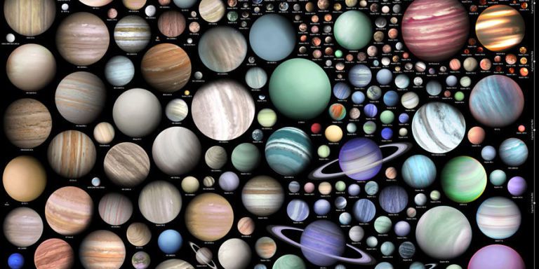
Planets are diverse!
(source: popularmechanics.com)
Planets are ubiquitous!
To view this video please enable JavaScript,
and consider upgrading to a web browser that
supports HTML5 video .
Because of Kepler , we found that planets are
virtually everywhere. We found systems that look nothing
like our own, and for the first time, we have proof
that our Solar System may not be a typical model. Here,
I'm showing a rather popular animation, the Kepler
orrery, which illustrates planets detected with Kepler
before the end of the mission.
Project 1: Structures and compositions of
tidally-distorted rocky planets
What are squishy planets?
Original idea (Hachisu 1986a,b): Use potential
theory and relaxation method to solve for the
shapes of stars in multiple systems
Stars modeled as polytropes, density $\propto$
pressure to some power $\gamma$
A rocky planet will act as a fluid on geological
timescales
Use a “modified polytrope” equation
of state (Seager+ 2007) $\rho = \rho_0 + A p^\gamma$
We attribute our method to the original idea of
Hachisu in 1986, who modeled the shapes of
rapidly-rotating stars and then stars in multiple
systems. These stars are pulled out of their
spherical shapes because of centrifugal and
gravitational forces. An important choice to make is
which equation of state, which relates pressure and
density, should be used for a particular model. The
polytrope is a classical EOS that is a good
approximation with a simple form. We modify Hachisu's
method in two key ways. First, we choose a modified
polytrope EOS that modifies the polytrope expression
for rocky material, which has nonzero density at
zero pressure.
What are squishy planets?
Second, we introduce an asymmetry in the geometry by
adding a point-source star at some distance from the
planet. Here, I'm showing the geometry of the system.
The planet is so close to the star that it is pulled
into a nonspherical shape along the planet-star axis.
There is a centrifugal force pushing the planet's
matter away from the axis of rotation, centered on
the star.
Methodology
Initialize with a guess density distribution
Compute the potential everywhere
Compute the enthalpy from the potential
Compute the density from the enthalpy
Repeat until convergence
The Hachisu method is essentially a relaxation
method, iterating between consistent densities and
enthalpies until convergence is reached. The math of
how the potential is computed gets a bit messy, so
I've omitted the formulas here, but, if you are
interested, you can look up the original Hachisu
papers or our own paper on arXiv.
PySquish implementation
Uses no internal parallelization — jobs are
submitted to slurm as array jobs
Python frontend, Cython bridge to C++ backend
Compiled-in grid resolution
Truncate the spherical harmonics series at a fixed number
PySquish was the first code I wrote to implement the
method I've described. It uses Python for some parts
and C++ for the more computationally-intensive parts,
with a Cython bridge between the two. The free parameters
in the model are two pressure parameters (central pressure
and core-mantle boundary pressure) of the planet, and
the distance from the star in simulation units.
Results from PySquish
This is one of the most interesting and important
results from PySquish. As the planet gets closer and
closer to the star, it eventually breaks apart, and
there is no equilibrium solution that allows the
planet to exist as a contiguous body in the orbit.
We might be curious at what orbital period this
occurs, remembering that Kepler's third law tells us
that there is a direct relationship between orbital
period and distance from the star. Where the minimum
orbital period occurs depends on the composition of
the planet, which is indicated by the colors on the
plot, where yellow planets are pure silicate and
purple planets are almost entirely iron. Finally,
the y-axis gives the radius of the planet. We
immediately notice a few trends. First, the silicate
planets break apart at larger radii than the iron
planets, which is intuitive because iron will not
distort as easily as silicate. As the planet gets
larger, it is also able to survive to smaller radii.
I'd also like to draw your attention to the vertical
white line. It indicates the properties of the
exoplanet KOI-1843.03, the exoplanet with the
shortest measured orbital period of 4.2 hours. We
see that, if this planet is sitting at the minimum
orbital period, it would be able to survive at
a moderately iron-rich composition. In this way, we
are able to infer a possible composition of the
planet without direct measurements.
Results from PySquish
Now, what happens as we change the composition of the
planet? Here, I'm showing the same plot, where iron
in the core of the planet has been replaced with
FeS, ferrous sulfide. Now, we see that KOI-1843.03 is
probably not consistent with this composition,
because only the upper limit radii overlap the
simulated curves.
SQUISHv2 implementation
Uses some pure MPI for task management
Uses PETSc for memory management (DMDA) and ODE solve (TS)
Compiled-in grid resolution
Truncate the spherical harmonics series at a fixed number
SQUISHv2 is the next generation of the PySquish code;
it is written completely in C and uses PETSc.
In my experience with this problem, there is a
trade-off between parallelizing over more cores and
distributing tasks among cores. Distributing the
problem over a couple of cores is pretty efficient,
though, and tasks can be split up among as many
pairs of cores as are available. I use a
“master” process that tells each of the
process pairs what to work on. This may not be the
best way to do this, so I'm open to any suggestions
for ways to improve. To discretize the problem, we
use a spherical grid in radius, altitudinal angle,
and azimuthal angle and expand the singular Poisson
kernel into spherical harmonics, again truncated at
a compiled-in number of terms. By thinking carefully
about storing previously-calculated values, we re-use
as many computations as possible and reduce the
computational complexity of the potential calculation.
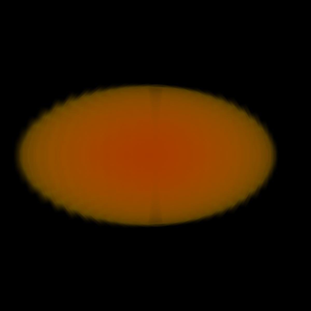
Volume render of a squishy planet
To bring home how cool these squishy planets really
are, I'm showing here a volume render of the full,
three-dimensional structure of a planet from our
sample. You can see the core and mantle of the planet
separately based on the colors, and the nonspherical
shape is very obvious from this point of view.
Where do planets form?
(inspired by Henning & Semenov 2013)
Many dynamical processes are active in protoplanetary
disks at any given time, some of which are shown
on this figure. (Explain each process)
Forming planets from dust
Dust grains collide and stick, bounce, or fragment
Grains are stickier if they have ices
Still have barriers to formation, so not a perfect theory
Astronomers have been theorizing on the origin of
planetary systems for quite some time. Our current
picture looks something like this: A molecular cloud
collapses and forms a disk shape because of
conservation of angular momentum. This disk is a
protoplanetary disk, named because we believe they
form planets. We believe that small grains collide
in the disk and stick together, forming larger and
larger pebbles. Small particles are sticky when they
have ice coatings, and it is this stickiness that
makes coagulation easier; once the boulder is large
enough, it has sufficient gravity to pull others into
itself. The problem with this theory is that meter-size
boulders are more likely to fragment or bounce on
collision than stick, and this is called the
“meter-size barrier”.
ALMA observes disks
(source: theverge.com)
ALMA, the Atacama Large Millimeter/submillimeter Array,
observes astronomical phenomena in the radio regime.
It is the premiere instrument for observing protoplanetary
disks and has allowed us to see details and substructure
that were impossible to see with older instruments. This
image shows the ALMA dishes, located in the Atacama
Desert in Chile. This telescope is like the one you'd
set up on your roof, with mirrors and lenses; instead,
it uses dishes and correlators to produce huge amounts
of data that are eventually turned into images using
computational techniques.
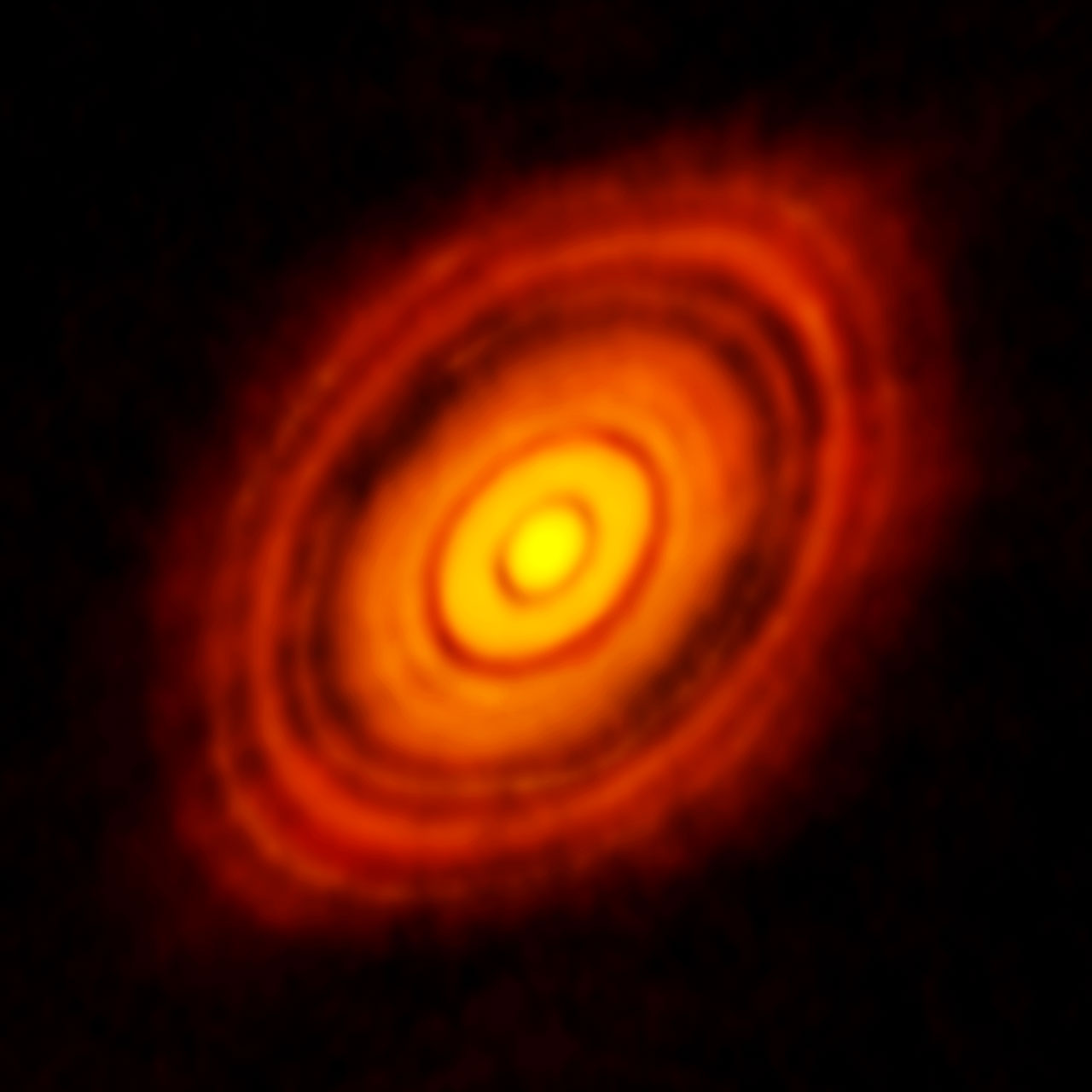
ALMA observes disks
(source: eso.org)
A striking example of an observed disk is TW Hya,
which was observed with ALMA after being observed
with older instruments. Virtually none of the
substructure, such as rings and gaps, were seen
in the original image.
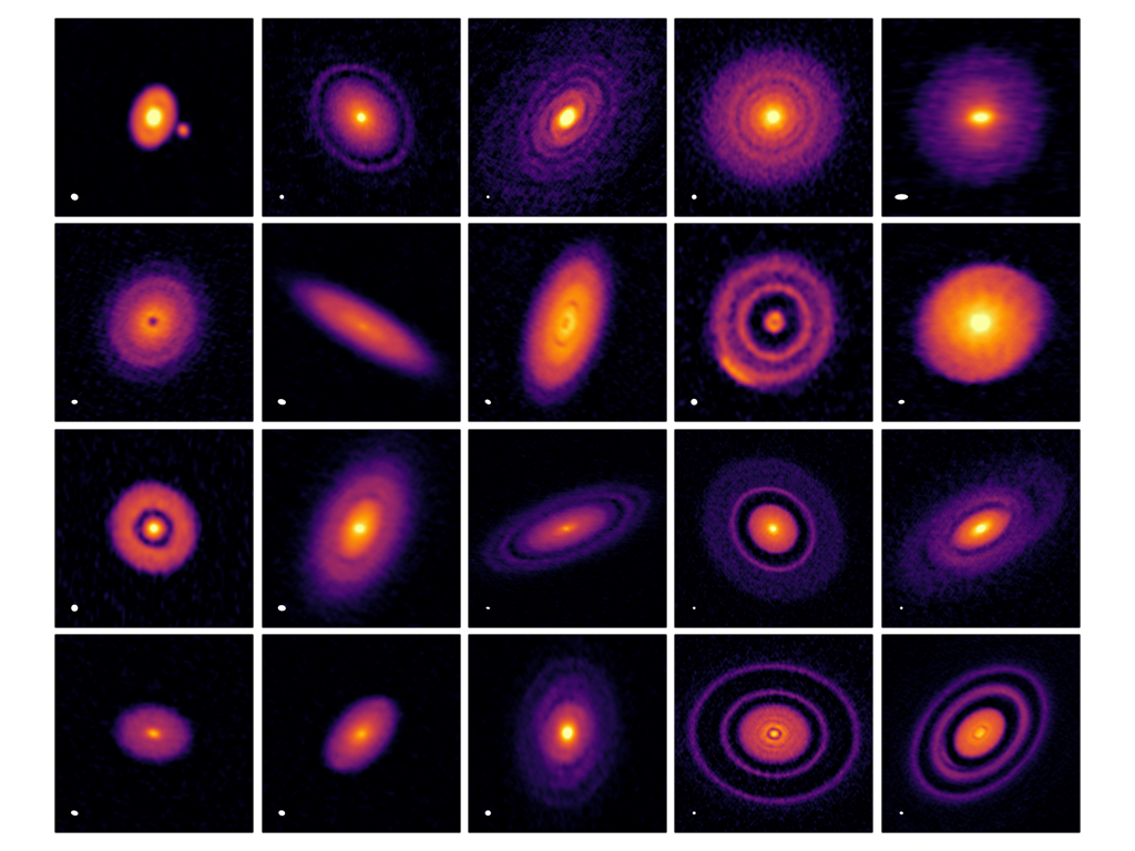
Even more substructure in disks
(source: almascience.eso.org, see Andrews, Huang+ 2018 and associated papers)
DSHARP, or the Disk Substructures at High Angular
Resultion Project, is a recently-published ALMA
project for observing the zoo of possible
substructures in disks. This image shows some
of the disks they observed, which have rings, gaps,
spiral arms, and anisotropies. This is important
to keep in mind, because, while we typically
assume for the sake of modeling that disks are
smoothly-varying in radius and azimuthally-symmetric,
they seem to be just as diverse as the planets they
produce.
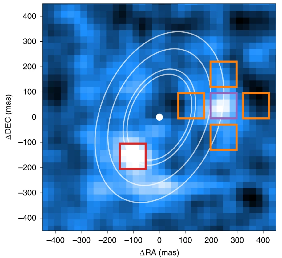
Observed early planets
(source: nature.com, Haffert+ 2019)
Even though we cannot observe planet formation in real time,
we have observed a few protoplanets embedded in disks,
which only serves to support our theory, even if some
details remain mysterious. Here, I'm showing the PDS 70
system from a recent Nature article. The authors claim
two young protoplanets embedded in the disk.
Formation environment is important
(inspired by Henning & Semenov 2013)
Now that we know a little more about how planets
form in theory, we can start to think about how
the dynamical processes change that picture. For example,
if a protoplanet migrates across a snowline, then it
will have a different composition than if it had
stayed fixed at one location.
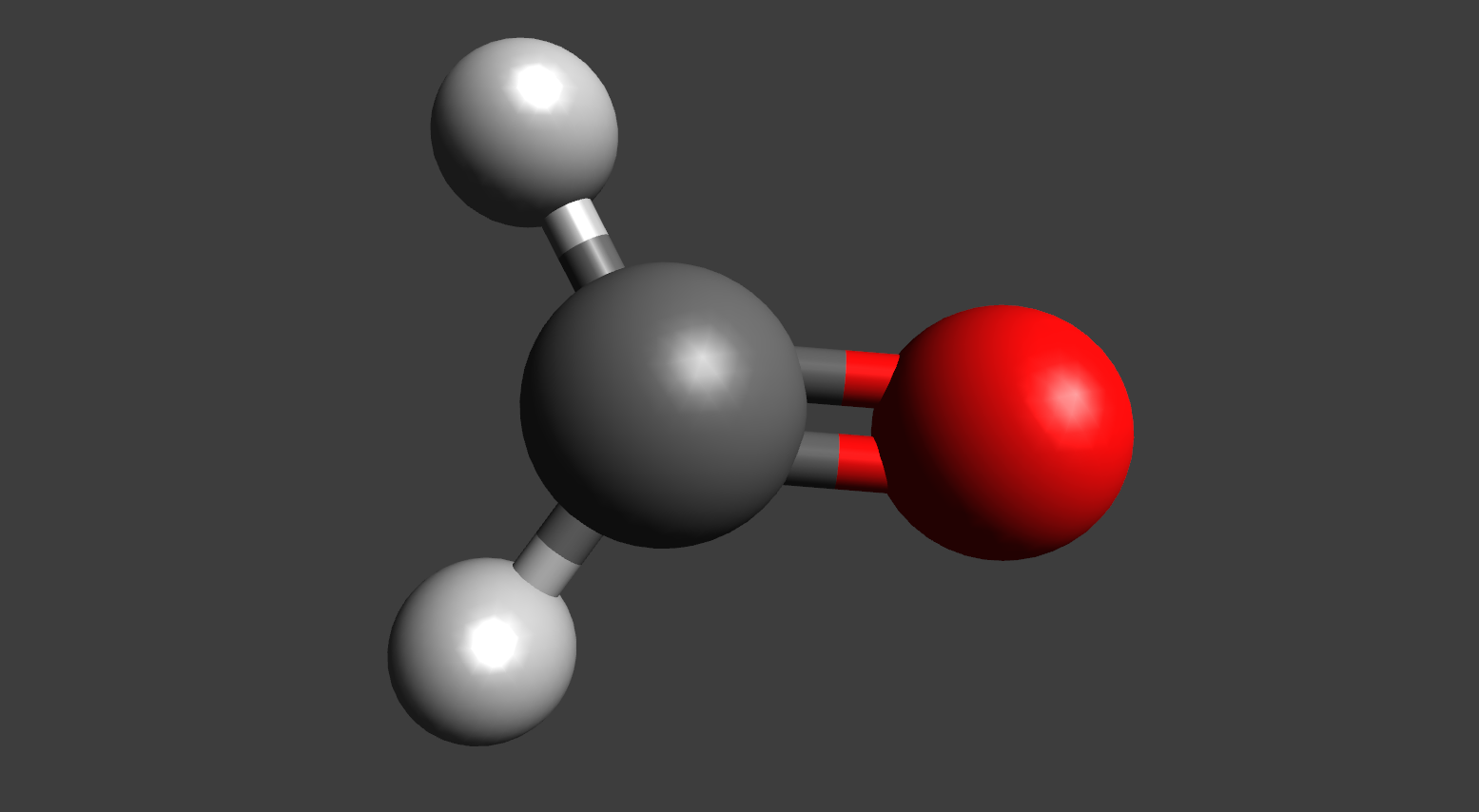
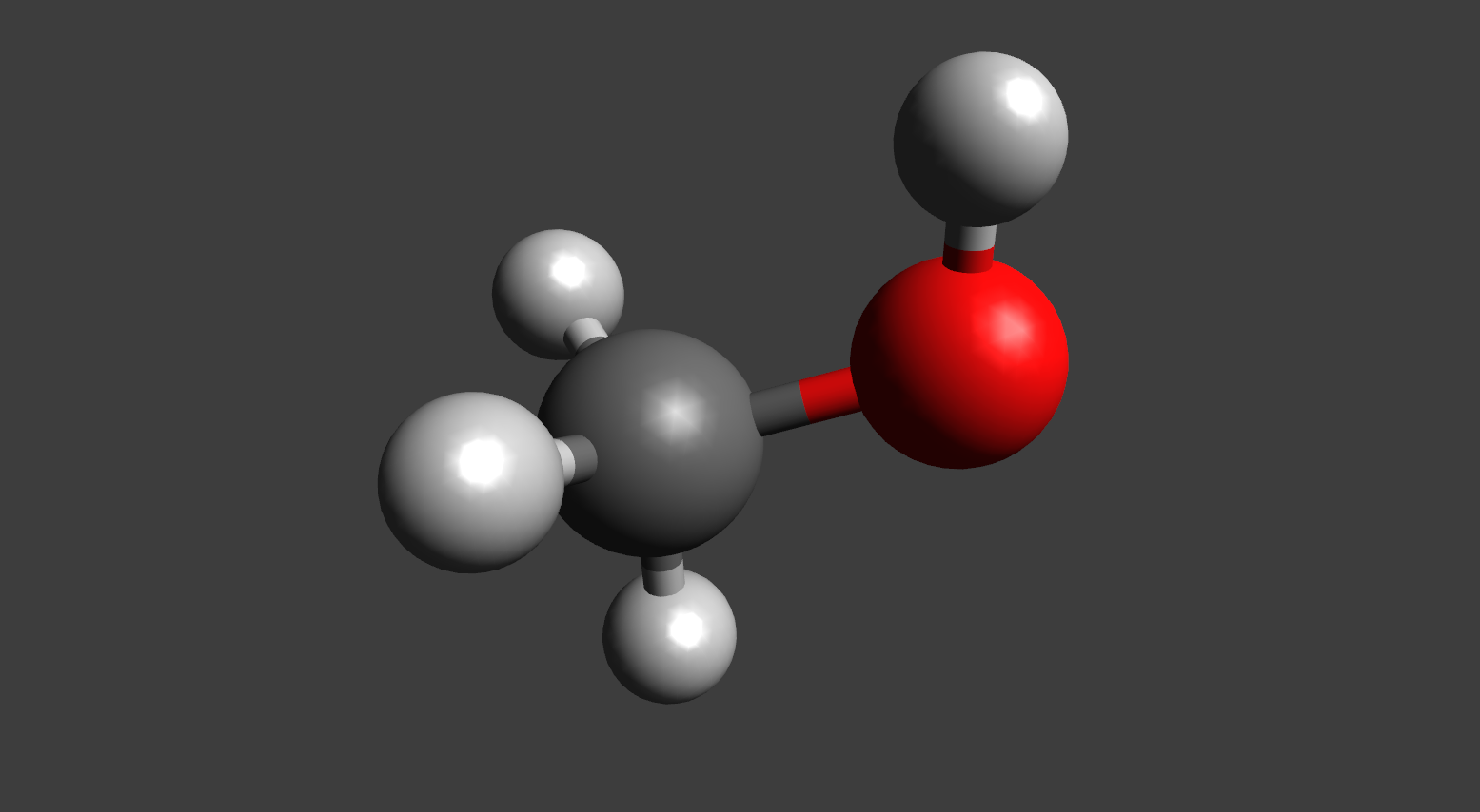
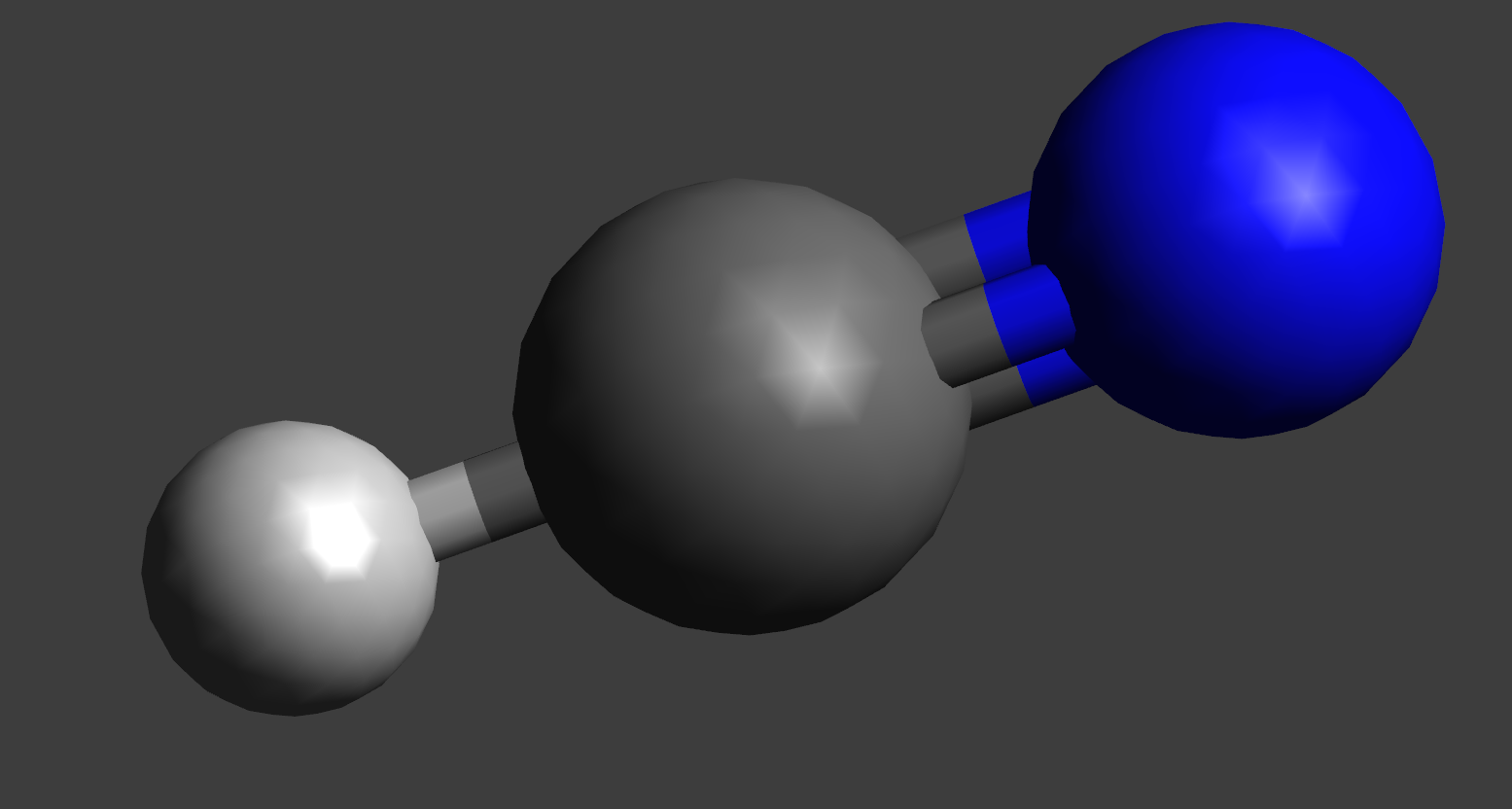
Disk chemistry
Formaldehyde
Methanol
Hydrogen cyanide
Astrochemistry differs from
traditional chemistry in that we deal with extreme
conditions and non-terrestrial molecules.Now, I've
hinted in the previous figures that the
composition of the disk depends on the vertical
height and the radial coordinate in the disk. Let's
discuss that a little more. Basically, where the disk
is highly irradiated, any molecules that could form
there break apart into atoms and ions. Under that
layer, where material is more shielded, there is a
warm molecular layer. Finally, in the cold midplane
of the disk, gas and grains coexist as a fluid
mixture. The next natural question to ask is,
what kind of molecules have we observed in disks?
Using radio astronomy techniques to observe rotational
transitions of molecules with a permanent dipole moment.
It's worth mentioning that we cannot observe
symmetric molecules like N2 because they
don't have a permanent dipole moment. On this slide,
I'm showing a few of the molecules that have been
observed in disks.
Disk chemistry
(courtesy of Karin Öberg)
In addition to knowing which molecules are
present in disks, we can spatially resolve disks
and know where the molecules are, too, modulo
projection effects. The figures I'm showing here
are spatially-resolved images of disks for a
particular molecule only; the alternative is
to image the continuum. You can see from these
images that substructure is even present in
individual molecules, so approximating the disk
as a well-mixed, homogeneous fluid is clearly not
founded by our observations.
Project 2: Coupling chemistry and accretion in a
protoplanetary disk
Problem statement
We want to know how accretion affects the chemistry
that occurs in disks to gain insight into the
compositions of planets that can form from the disk
material.
I hope my introduction got you thinking about
how the physical processes in a disk might affect
the chemical processes in disks. For this project,
I just want to focus on one physical process:
accretion. How does accretion affect the chemistry
of a protoplanetary disk?
Global solution
Can do a single, “global” simulation
of disk chemistry
Pros:
Can incorporate as much physics as needed
Cons:
Very computationally expensive!
If we have $M$ species and $N$ computational
cells and cells are not independent, would
need a $M N \times M N$ (sparse) matrix to
solve for all chemistry at a single timestep
Examples given in Haworth+ (2016)
How might we go about solving this complicated problem?
One possibility is to solve for the disk surface density
and composition at all times, at all radii, all at once.
This would allow us to incorporate as much physics as
we want, including all the processes I've mentioned today
and even more. But we don't have the computational power
to do so for a dense sampling of radii (plus, spoiler
alert, there's a better way!).
Alternative: reduce chemical network
Can choose a subset of “important”
reactions to reduce number of reactions and
species being considered
Pros:
Can incorporate as much physics as needed
Cons:
Lose chemical insight
Chemical network reduction is a science/art itself!
On the other hand, we could reduce our chemical network
by including only the most important species; the full
network in what I will describe has about 600 species.
However, we would lose chemical insight by doing this,
and reducing a chemical network in a meaningful way
is practically a thesis in itself.
Alternative: reduce physics
Can reduce the physical processes considered
Common approach is to assume that disk material
is not moving radially or vertically
Pros:
No loss of chemical complexity
Cons:
Missing (possibly) important effects of
dynamic processes
Finally, we could reduce the physics, which would allow
us to include as much chemical complexity as possible,
but we would miss out on the dynamic processes that
we suspect may actually be very important for that
chemistry.
Alternative: local simulation
Solve for accretion tracks self-consistently and
follow chemistry along tracks
Pros:
Under some assumptions, no compromise
between chemistry and physics
Approximately equal computational load to a
static model
Can be built upon in future work
Example: Heinzeller, Nomura, & Walsh (2011)
So we don't do any of that. Instead, we do a local
simulation, which assumes no mixing between computational
cells but allows us to have arbitrary chemical complexity
in each cell and we can incorporate as much physics
as we like as long as we are creative enough to keep
the key assumption of no mixing.
Surface density
$$ \frac{\partial \Sigma}{\partial t} - \frac{3}{R} \frac{\partial}{\partial R} \left[R^{1/2} \frac{\partial}{\partial R} \left(\nu \Sigma R^{1/2}\right)\right] = 0 $$
From Lynden-Bell & Pringle (1974) and Pringle (1981)
By combining the Navier-Stokes and mass continuity equation, we find a diffusion-type equation in surface density $\Sigma$
I'm going to show this equation but not go into any
detail about its derivation. If you are interested,
I've listed the original papers here. There's also a
rather excellent derivation in the book, Principles
of Astrophysical Fluid Dynamics that uses the
Navier-Stokes equations. This equation governs the
time evolution of the surface density of the
protoplanetary disk. Surface density is just the
mass density integrated over the height of the disk.
I solve this equation using the PETSc TS interface
with Crank-Nicolson timestepping scheme and simple
finite differences discretization of the spatial
derivatives. This turns out to be sufficient for
our purposes.
Chemistry post-processing
Consider chemistry in a “box”
$$ n_i + n_j \rightarrow \cdots $$
$$ n_{j1} + n_{j2} \rightarrow n_i + \cdots $$
Chemical network: reactions with rates $P_j$ and $R_j$
$$ \frac{\mathrm{d} n_i}{\mathrm{d} t}\bigg|_V = \sum\limits_j P_j n_{j1} n_{j2} - n_i \sum\limits_j R_j n_j $$
Once we have the surface density, the trajectory of
any given parcel of gas is simply a function of its
initial radius, and it turns out that these
trajectories don't cross! Now, we're ready to do
chemistry. We only consider two-body reactions, since
three-body reactions are very rare at the relevant
densities. These are the coupled ordinary differential
equations that correspond to a single chemical species,
and there are roughly 600 species and 6000 reactions
in our chemical network. For integrating these
equations, I use SUNDIALS with the BDF integrator
and PETSc's MUMPS interface for preconditioning.
Tracks through the disk
(source: Price, Cleeves, & Öberg, 2019, in prep.)
To give you an idea of how the tracks actually look,
here is a plot from the paper in preparation showing
how various variables vary over one of these tracks
that spiral in towards the central star.
Does accretion affect chemistry?
(source: Price, Cleeves, & Öberg, 2019, in prep.)
So does accretion affect chemistry? Yes, it really does!
Acknowledgements
Used in this presentation:
reveal.js ,
highlight.js ,
Nord ,
Nord for highlight.js ,
Inter font ,
Avogadro molecular editor ,
Inkscape
Used in the projects:
PETSc ,
SUNDIALS ,
OSPRay ,
Embree ,
ISPC ,
TBB
Resume presentation
Applications of PETSc to open questions in planet formation theory
Ellen M. Price
Center for Astrophysics | Harvard & Smithsonian
PETSc '19, 7 June 2019
Hi, my name is Ellen Price, and I'm a rising fifth-year
graduate student at the Center for Astrophysics |
Harvard & Smithsonian, a collaboration between
Harvard University's astronomy department and the
Smithsonian Institution. Today, I'd like to
talk to you about how I've applied the PETSc software
to my research in the field of planet formation.
Before I get started, though, I'd like to thank the
conference organizers for inviting me and putting
together a terrific event.