Hectospec Observers Reference Manual

Figure 1. Hectospec focal surface.
2 The
astronomer’s duties are limited to preparing the robot
configurations for observing and taking data with the bench
spectrograph. MMTO and SAO staff will
prepare the
spectrograph for observing and will fill the dewar. 1.
Run
the
spectrograph/CCD acquisition
control software 2.
Annotate
the
data logs (now under
automation), with comments on conditions, data quality, problems
encountered,
etc. 3.
Check
the
operation of the spectrograph/CCD
at the beginning of the night, and monitor readout noise, spectrograph
focus,
thermal flexure, etc. Normally, the
actual focusing would be done by the robot operators, Perry and Mike,
who would
also fill the CCD dewar. 4.
Be
knowledgeable about the fiber assignment
code "xfitfibs", in particular with regard to the restrictions on
rotator position and guide star selection, to the extent of being able
to run
the program at the telescope should the need arise. 5.
Be
knowledgeable about the normal sequence
of operating the positioner and acquiring fields, so that when problems
with acquiring a field occur, the
robot
operators can be advised as to how to proceed (e.g., moving on to
another field
because of poor guide stars). This would
not include actually operating the positioner; that task would remain
in the capable
hands of trained personnel. 6.
Do
quick look
reductions of data as it
appears, checking for overall quality, and in particular insuring that
the
spectra fulfill program goals. E.g., are objects detected at all
(coords ok?),
are objects underexposed or overexposed, etc. 7.
Help
make
decisions regarding the queue
during times of marginal weather or seeing, choosing targets from the
nightly
list. Normally, the nightly observations
are scheduled by the queue manager (Caldwell at this time). To
aid the
on-site astronomers, each group
with Hectospec time will be expected to supply a brief summary of their
data
and calibration requirements. Please
submit your configuration files at least 10 days before the run starts. The Hectospec bench spectrograph has 3
motors that
need to be
powered up and initialized at the beginning of a run, and often at the
beginning of each night as well, if power has been shut off for safety. These motors control the CCD dewar focus
stage, the grating angle, and the High Speed Shutter (mounted on the
fiber
shoe). The CCD electronics control and
the dome calibration lamps must also be powered up and initialized. A
suite of three Linux boxes operate the robot positioner, the bench
spectrograph, and the CCD camera (several other computers do work as
well, but
will remain nameless here). The instrument rack on the 2nd
floor must be powered up as described above Figure
8. Spice
Startup page. Use this to initialize
software and home the three spectrograph motors. After
this process is complete, return to the
startup page for observing. There
are several tabs in this menu, which can be selected as needed. For the first start of a new observing run,
select “Startup,” which is used to
initialize the spectrograph. The
sequence is: Start
Pulizzis, Start Rack (wait 2 minutes) Start Bench, Home
Bench, Start CCD, Start DomeCal. The CCD
temperature is controlled via a heater in the CCD dewar.
If the CCD electronics have been off for a
while, say since the previous morning, the temperature will be colder
than
nominal (perhaps as low as -135 °C) and thus the heater will come on
for an
extended period till the temperature reaches -120 °C.
Thus, for critical measurements, you may wish
to monitor this temperature until it reaches nominal, as shown on the
Spice
upper panel. The
next tab allows configuration of the bench, e.g., changing the grating
or
grating tilt. Press "ConfigBench" at the begining of the
Hectospec run, or if you have changed either the grating or operating
wavelength. Also on this page, enter the observers’ name. The
Program ID
("Propid") and the PI values will be entered automatically when a
configuration is selected by the robot operator. For testing
purposes,
the telname may be set to "Test", the instrname may be
set to "test", or the detname may be set to "test"
or "specn". Nomally, these should be set to
"mmt_f5_adc", "hectospec" (or "hectochelle"), and
"specs". If the telescope is off however, and you want to take
some test data (darks for instance), then set the telname to "test",
lest an error occur. The grating,
binning and/or the wavelength setting is chosen in this
tab as
well, with only the allowed choices being available in the pull down
menu. The configuration loaded by the
positioner
software limits the choices for these parameters, thus minimizing the
possibility of mistakes. The “Standard Ops” page provides exposure control
for the
CCD, as well as limited control of the spectrograph and the dome lamps. The control is based on the ICE system. Figure
9. Spice
Standard Ops page for taking spectra. If
the box on the lower left above the Pause button is selected, a pull
down menu
of observation types appears to select the exposure type. An
exposure is taken by selecting a type of exposure from the pull-down
menu
(shown as obect1 here). Choices include “object”, “comp”
etc. The
number of exposures and the exposure time are taken from the columns to
the
right Go box (green before an exposure, red during an exposure
as shown
here). Click on Go to start an exposure. The user is
prompted for a
title. The Exposure box and queue status shows the
progress. Upon
readout completion, a beep is issued and the file is automatically
displayed
into a ds9 window (called “ds9spec”). To stop an exposure, first pause
it. The rest of the tabs are described below. OBJECT:
prompts for a title, opens the shutter, writes “object” as
imagetype in the
header. SKYOBJECT:
prompts for a title, opens the shutter, writes “skyobject” as
imagetype in
the header. Used for blank sky fields taken between object fields. SKYFLAT:
prompts for a title, opens the shutter, writes “skyflat” as
imagetype in
the header. Use this for twilight sky exposures. COMP:
prompts for a title, opens the shutter, writes
“comp” as imagetype
in the header. Use this for dome exposures of HeNeAr etc.
Startup
the dome lights with the appropriate button for HeNeAr,
exposure times
of about 5x300 seconds are recommended, multiple exposures are useful
to
eliminate cosmic rays. With the PenRay HgNeAr combination,
shorter
exposure times may be used (30 seconds or so). DOMEFLAT:
prompts for a title, opens the shutter, writes
“domeflat”
as imagetype in the header. Turn on the dome continuum
lamps.
For the dome continuum exposures with hectospec, an exposure time of 2
seconds
is recommended. Shorter exposures may suffer from shutter
vignetting, and
thus would not be useful for throughput corrections, though the files
should
still be ok for pixel-pixel flattening. QFOCUS:
used for SPEC only. Enter the number of exposures desired, the
center focus value, and
the
focus step between exposures. Good values for SPEC are 7,
4, and
-0.04. This routine will take a sequence of exposures, at the requested
sequence of focus values for the spectrograph, which can then be
analyzed. Typically, one uses the dome calibration
PenRay
lamps for this purpose, though night sky emission lines work well
also. The
exposure can also be done while the mirror is covered.
This
program uses the grating in zero order, and the charge is moved between
the
exposures, thus only one file is produced. The image will have
one spot
per fiber, per exposure. So the image will have 300
rows of n
spots, where n is the number of exposures. Bearing in mind that
the
in-focus images are not Gaussian but rather flat-topped, a script has
been
written that analyzes the data frame and produces a plot. In an
iraf
window, type this command: qfocus filename. A plot in gv
will
be produced showing image concentration as a function of focus
position.
Different fibers are shown as different symbols. Higher
concentrations
are better. Once you
have
determined the focus, you still must set
it using the Focus tab. FOCUS:
used for CHELLE. nter the number of
exposures desired, the starting focus value, and the focus step between
exposures. This routine will take a sequence of frames, at the
requested
sequence of focus values for the spectrograph. Typically, one
uses the
dome calibration HeNeAr or ThAr lamps for this purpose, though night
sky
emission lines work well also. FOR
CHELLE : the step should be -0.05, exposures 120s, and take 7 of
them The program FOCUS.sh N,
will
extract information from the most recent
N focus exposures To run this, type ./FOCUS.sh in a terminal window
(not in
iraf). Another program will display the
focus files in tiled images on ds9. In this case, type display_focus N. DARK:
prompts for a title, does not open the shutter, writes “dark” as
imagetype
in the header. There are light leaks around the shutter, so darks
should
be taken with the chamber lights off. The dark rate is extremely
low, and
in normal circumstances does not need to be measured. Be aware
that the
fluorescent lights in the spectrograph room will elevate the dark count
significantly for about an hour after they are turned off. BIAS:
prompts for a title, leaves shutter closed, writes “zero” as
imagetype in
the header. There is some structure to the bias, so we recommend
taking a
handful of these at the beginning of the night. The autoops tab is
not
described here.
The focus tab is used after determining a new focus. Enter the
correct
value next to new focus, click on apply and set. The next tab shows the calibration
lamp
status. The lamps themselves are usually controlled in the
standard ops
tab, but this tab shows the details of eack kind of lamp. The start/stop tab allows control of the
many
software
servers in the system. Select the action wanted at the middle
right
("restart, start, stop"), then click on the button desired to the
left (e.g., domecal up). The shutdown page allows one to shut
down the
spectrograph
and wide field corrector. Normally done by the robot operators. The
comment window is used to create and maintain the data logs,
which are
mostly automatic. The one thing the observer can add is a comment
when needed.
In particular, it useful to comment on the seeing and cloud presence
during the
night, and any problems with particular files. To do so, first insure
that the
correct data has been selected (recall that we use the UT date). To
comment on
an existing file, click on its name in the right panel. The basic
information
will appear to the right, and you can now type into the comments
panel.
Click on Save Changes. To edit an ongoing exposure,
click on
Open Current and then enter comments. To view
the data
logs, click
on the sunburst button at the bottom right. A postscript file is
created and
the displayed using gv. Exit gv using q. Very lengthy comments will be truncated. Type what you
need, display the result, and if necessary, move the excess
verbiage to the comments for the next exposure. Copies of these
logs may be viewed by non-attendant astronomers at arond noon EDT at this
web site.
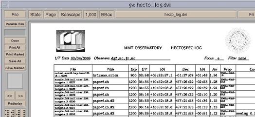
Figure
12
Example data log. The A/D converter is 16 bit, so
saturation occurs
at
65536. There are 2 amplifiers per CCD,
and thus the data are stored in FITS extension format, with 5
extensions (0
being the main file header). Among other
things, this means that in iraf, you will occasionally have to refer to
the
file as filename[1] or [2], say when using imheader (though not
imexamine). The data from the different amplifiers
are not
flipped to
the same orientation before writing to disk,
but the header keywords allow ds9 to display the files
correctly. We hope
that all the file keywords are correct, and that programs like
IRAF’s mscred will work, but we can’t
guarantee this at this time. The SAO
version of NOAO’s mscdb package must
be installed to use mscred. As already written, the data files are
stored in
directories
of the format /SPEC/ year.monthday (or
CHELLE/ year.monthday . The files are
also archived both on the local computer as well as back in The fiber mapping files (“filename_map”)
are
stored along
with the data files. This information is
also stored in the FITS file. Each new file is automatically displayed
into the
active
frame of ds9 (named spec9 here to avoid conflicts with other ds9
programs that
may be running). To load files off
the
disk, select FILE:OPEN OTHER: OPEN MOSAIC IRAF, and then find your
directory
and filename. You may load files into
different frames via creating a new frame: FRAME:NEW.
Run through frames via Tab. Do not
use mscdisplay in IRAF. The contrast can be changed with the
right mouse
button. For
further contrast levels, select Scale:Scale Parameters from the top bar menu.
You’ll get a histogram of the data – high and low values may be
selected by
moving the red and green vertical lines with the mouse. Note that the files are shown with blue
on the
left, thus
requiring the XY coordinate system to be non-standard.
Image coordinates refer to individual
extensions (one per amplifier), and thus start over when crossing into
an new
extension, while the detector coordinates refer to the combined image. The default display also excludes the
overscan areas. To see these, select SCALE and turn off DATASEC. However, some of the overscans will display
over that from the next image extension… Imexamine works as is with these files;
there is
no need to
use mscexamine. Make sure
you start up IRAFin a xgterm
window. The data obtained by CfA PIs will be
reduced by
the
Telescope Data Center (TDC) unless the spectrograph operation mode is
inconsistent
with the standard pipeline or unless the PI wishes to reduce his or her
data. For non-CfA users the TDC will
make the pipeline software available.
Check the TDC website (http://tdc-www.harvard.edu/
) to download this software. Doug Mink (dmink at cfa.harvard.edu) may be
able to
provide advice about this software in case of difficulty.
Nelson Caldwell is very familiar with the
operation and characteristics of the spectrograph, and has a good deal
of
experience with data reduction. He is
willing to provide a limited amount of help to users; he may be
contacted at caldwell at cfa.harvard.edu".
All Hectospec or Hectochelle data will
be archived
nightly
by the TDC. A
fairly
fast
method of extracting all 300
fiber spectra from Hectospec images (or 240 spectra for CHELLE data) is
provided
by a command that runs a series of PERL and IRAF scripts. The input is
a series
of raw images, which are processed as described in this document
<http://cfa-www.harvard.edu/oir/MMT/MMTI/hectospec/hecto-reductions.htm>.
The calibration files used are stored in a subdirectory, and may need
to be
remade for every observing run (but not every night). The output is a
FITS file
containing wavelength calibrated, sky-subtracted spectra in multispec
format
(for CHELLE no wavelength calibration or sky subtraction is done)..
The
program currently runs on lewis. Here
is what you need to do: 1. Open an xgterm , with xgterm
&. You may resize the font via
shift-middle mouse
button. Start up IRAF with cl. 2.
You'll
need to know the names of the files you want to combine. The IRAF
command
ldata will list the files in the current data directory, or you
can look
at the data logs. The output files will be written in
the
current directory. 3.
For
multiple files, the program detects the cosmic rays by comparing
images,
and interpolates across them in individual frames, The frames are
then
averaged together before extraction begins. For a single
exposure,
the cosmic rays will not be deleted. 4.
In
the IRAF window, you would type :
qspec
file1,file2,file3 where
the files are of the form listed from the
data command, e.g., halostar9:30pm_1.1121.fits.
The
.fits extension is
unnecessary. The
files must be separated by commas with no spaces. Alternatively,
one may reduce the most recent
file or files via: qspec
lastN where
N is optional or the number of files of the
same object you want to combine.
Finally, you can extract older spectra via a command like: qspec
file1,file2
“2006.1010” which
would extract and combine files file1 and
file2 from the 2006.1010 directory. 5.
The
program takes 1-3 minutes. The files used in the process are then
listed,
along with the names of the output files. If the output file existed
already,
the program will prompt for deletion. 6.
To look at the
spectra, use splot (you may
need to load imred and then specred first, though they are supposed to
be
loaded automatically). To run through the spectra one by one, use the (
and ) keys. The X and Y scales have been
fixed to display low signal spectra well; to scale to the entire range
of the
spectum, type w and then a while viewing a spectrum. To
smooth,
type s. 7.
At
the
beginning of each Hectospec run, and certainly if the fiber shoe has
been moved
from Chelle to Spec, a crude wavelength adjustment must be made. Inspect the extracted spectra which have not
been skysubtracted from any of your images.
Using splot, determine the wavelength of the brightest night sky
line
whose wavelength is supposed to be 5577A (but which may be off a little
because
of the problem we are about to fix).
Subtract the measured wavelength from 5577 (i.e.,
5577-wave_observed).
In Spice, select the configure tab, and locate the quick
look
wavelength offset window. Note the wavelength offset in this window,
and add
the offset you just determined to the existing value. Click on save. Now rerun the extraction. The skysubtraction
should work properly now. Trouble
may ensue if there are no sky fibers in apertures 1-150 or 151-300. A
ds9 regions file can be brought up to identify all the apertures and
which
fibers they correspond to. Click on regions, and load regions, and
select the
file /h/spec/specaps.reg. We currently have available a 270
groove/mm
grating blazed
at 5200 Å, and a 600 gpm grating blazed at
6000 Å, both purchased from David
Richardson Grating Laboratory. The
spectral coverage, spectral resolution, anamorphic magnification,
grating
angles and RMS image diameters for these gratings and as well as a possible 1200 gpm grating, all set up with Ha as
the central wavelength, are shown below.
The spectral coverages in this table refer to the nominal 3400
pixel
format. However, the image quality holds
up quite well over the whole 4608 pixel format, and the full spectral
coverage
is ~1.35 times that shown in the table.
Remember that second order contamination may be an issue for
some
applications. Currently, we do not have
order blocking filters.
The spectral resolutions quoted are as
measured with arc lines, with the first number referring to wavelengths
around
4500 Å, while the second refers to 7000 Å. Ruling Density (gpm) Spectral Coverage (Å) Spectral Resolution (FWHM Å) Anamorph. Mag. Angle of Incidence Angle of Diffraction RMS Image Diameter (pixels) 270 4488-8664 5.8-5.0 1.06 22.83 12.17 1.3-1.8 600 5609-7522 2.2-1.9 1.14 29.41 5.59 1.3-1.8 Figure
15. The efficiency of the 270 line grating Figure
16. The efficiency of the 600 line grating. The Hectospec optical layout is simple
enough that
very high
throughput can be achieved if good reflective coatings are used on the
mirrors
(2 surfaces) and good antireflection coatings are used on the lenses (6
fused
silica surfaces). We have used the same
dielectrically-enhanced silver reflective coatings and Sol-gel
antireflection
coatings that we used in the efficient FAST spectrograph.
Our predictions for Hectospec's overall
throughput with the 270 line grating are shown below.
The column labeled “Add. Fiber Losses”
includes FRD, end reflection losses, and the losses from misalignments
of the
fiber axis with respect to the chief ray at the f/5 focal surface. This table does not include aperture
losses
at the fiber input, which will depend on the seeing and the quality of
the
astrometry of the targets and the guide stars. Wave Mirror Refl. (2 surf) Lens Thrput (6 surf) Fiber Thrput (26 m) Add. Fiber Losses CCD Effic. Grat Effic. Tele Refl + 10 cor surf) Final Throughput, Hectospec plus Telescope Optics 3650 0.90 0.89 0.70 0.80 0.66 0.80 0.37 .66 0.06 4000 0.90 0.92 0.80 0.80 0.80 0.80 0.49 .70 0.12 5000 0.91 0.98 0.90 0.80 0.85 0.80 0.66 .79 0.23 6000 0.92 0.98 0.94 0.80 0.80 0.80 0.61 .79 0.21 7000 0.92 0.98 0.96 0.80 0.75 0.80 0.53 .75 0.17 8000 0.92 0.95 0.98 0.80 0.60 0.80 0.43 .66 0.09 9000 0.92 0.91 0.98 0.80 0.30 0.80 0.37 .65 0.04 We can compare
the throughput predictions
with
measurements
of a spectrophotometric flux standard star BD+284211 in 1″ seeing. BD+284211 was stepped across a fiber entrance
aperture to find the position where we detected the maximum flux. For an apples to apples comparison we need to
correct the
measurement for the aperture loss. The appropriate aperture correction for
the plots
above
(measured with Megacam images) is about 1.7 (ratio of flux within a 20″
diameter aperture to the flux within a 1.5″ diameter aperture). Therefore, the peak throughput for light that
hits the fiber aperture is about 17% (to be compared with the
prediction of
23%) . If we average over wavelength,
the measured throughput is about 75% to 80% of the predicted numbers. We present two “real-world” performance
plots: the
SNR pixel-1
for a 45 minute exposure as a function of aperture magnitude, and the absorption line SNR (1+R) for 45
minutes of exposure as a function of aperture magnitude. Figure
18. The signal-to-noise ratio per pixel for a 45
minute exposure as a function of aperture magnitude (1² diameter
aperture.) The SNR per pixel is ~26 at
R=21. The relations for 4500 Å and 8500 Å
have the
similar slopes, but show a SNR per pixel of ~9 at an aperture magnitude
of R=21
for the same exposure length.
Improvements in sky subtraction techniques may allow improvement
at 8500
Å . Analysis and plot courtesy of Daniel
Eisenstein. Figure
19. The absorption line cross-correlation
signal-to-noise ratio ~(1+R) for 45 minutes of exposure as function of
R aperture
magnitude (2.6²
diameter aperture). All of the 1974
galaxies in this plot had reliable redshifts.
The SNR ratio shown here is reduced somewhat by the use of
templates
from the FAST spectrograph. Better
cross-correlation templates will be created.
Courtesy of Michael Kurtz. This list is meant for the attending astronomers. If the equipment is all ready, or if the run is underway,
skip to
item 8.
2
What to expect at the Telescope
The observer’s main responsibilities are to
prepare the
fields for observation with the planning software, to take data with
the
spectrograph, and to help replan observations during the night if
conditions
require a change. Observers should
be
familiar with the planning software and the instrument constraints
described in
the next few sections.
The most common error that we have encountered is
poor
choice of guide stars, including guide stars that are too faint or that
are in
fact compact galaxies. We strongly
recommend guide stars brighter than R=15.5.
Observers should use the preview feature in the XFITFIBS
software to
eliminate galaxies.
Hectospec will be operated in queue mode. Observers
may therefore expect to receive a
fraction of the clear observing time during each run equivalent to
their
fraction of allotted time during that run.
We try, if at all possible, to observe some of the officially
scheduled
observer’s fields during their run. If
observers are not prepared with valid configuration and catalog files,
observations cannot be made.
Currently Nelson Caldwell is responsible for queue
scheduling. Nelson attempts to review
the submitted files to see if they are valid.
3
Duties for Hectospec Observers
Observer
Responsibilities
4
Fitting Fibers to Targets, Running Xfitfibs
(1)
The PI makes a catalog of objects, which may be ranked in
preference. The catalog must also include guide stars on the
same coordinate system. Guiding is done at the edge of the Hectospec
field,
not on the surface where the object fibers are positioned.
Thus, there are very stringent requirements on guide
stars by the small area of sky available and the limited range of
magnitudes
allowed by the TV cameras.
The
2mass and GSC II catalogs can be used where an observer catalog
is
minimal in stars. In that case, the program tmcguidestars
should be
used. This program searches the 2mass catalog for coincidences with the
observer catalog, and computes a coordinate
transformation. 2mass and GSC II stars are selected in the field,
transformed to the observers' catalog coordinate system, and added
to the catalog. Note: the target catalog must have some stars in
common with the 2mass catalogs. You might need to add stars to
insure that, even if you don't intend on observing them. Bad News tmcguidestars is not
yet ready
for export. It does run on CfA computers, in a command line mode.
External projects should contact instrument scientists if they need
help with guide star selection.
cfa-www.harvard.edu/~john/xfitfibs/
and runs the config program for approximate dates of
observation. In this process, guide stars are checked for
suitability using a number of criteria (magnitude range, not a
galaxy, no neighbors, etc).
(3)
xfitfibs requires information such as date and length of
observation, number of exposures, ranking of config, and for Chelle
observations, the filter and binning needed, all which will be
used in scheduling.
The output of the program is a number of files which
would now be sent to a CfA computer for human checking, via the
button Submit . After they are checked at CfA,
the configuration files are sent to a computer at the MMT.
(4)
The configuration file is modified at the telescope a few minutes
before the observation
takes place,
in order to update positions, rotation angles, random sky selections,
and guide stars.
4.1
Brief Instructions for
Xfitfibs
4.1.1. Make a
catalog
ra
dec type
but it's probably better to have more:
ra
dec
object rank type
mag
A sample catalog would look like:
ra
dec
object rank type
----------- -----------
---------- ---- ----
0:40:30.289 41:16:08.73
008-060 1 TARGET
0:40:31.566 41:14:22.54
010-062 1 TARGET
0:54:58.594 43:05:22.298
guide
0:54:59.146 39:03:36.815
guide
Note the row with dashes (also tab delimited). "guide" indicates the
guide stars, located at the end of the file. In this case, the
guide stars have no rank or object name (but the tabs are there).
The starbase suite of programs may be downloaded at
http://cfa-www.harvard.edu/~john/starbase/starbase.html
The command check is
useful top run on your catalog to see that the format is valid (type
"check < mycatalog"; no message means that the catalog is
valid). The command fldtotable
will convert an ascii table to starbase (see the help pages).
It is nothing
short of essential that the targets and guide stars be on the same
coordinate system.
4.1.2 . Run Xfitfibs
4.1.2.1 Load catalog and select field centers
4.1.2.2 select candidate guide stars
Click on Fit Guides tab,
then begin fit.
The number of guide stars will appear at the far right of the fld table
row. A red background means too few stars available. You may have to
move the circle center or change the mag limit on the guide stars (at
the peril of them not being seen at the telescope).
It may also be the case that the rotator angles are red, even though
there are enough guide stars. In this case you can change those
angles by clicking on "toggle guide
annuli", going to the drawing window clicking on the (faint) red
circle at the ends of any of the 3 annuli and dragging the annuli
around until r0,r1 and r3 are green.
Next you need to classify the guide stars to remove double stars,
stars that are too faint, and plain old galaxies. Click on
"classify candidate..."
After a while a message will come back with the results. Some stars may
be rejected. Click on ok to rerun the guide star selection.
You can view the guide stars by bringing up the "Guide" window.
Use view to elect each config
in turn.
Clicking on show, will
start up ds9 and display all the guide stars in different frames. Nixed
stars may also be seen by using view. If you are left with no
guide stars, you may try to lower the faint mag limit in the parameters
menu, but please advise us that you have done so, and expect some
trouble at the telescope.
4.1.2.3 Fit fibers.
Click on fit fibers, if your
objects have a ranking system, then select rank, otherwise don't click on it.
Make depth=7. If you are
configuring
for Chelle, click on that as well. Now, begin fit.
Note that all the field centers you have entered in the fld table are
fit at once, such that no target is assigned more than once. If
you create two different output files from the same catalog, by running
xfitfibs at different times with different field centers, then you may
have duplicates.
Check to see that you have fit the number of targets you expected,
otherwise, change your sky fiber numbers in parameters. Ranking
of targets may be changed by using the rank window. See the
details in the help page.
4.1.2.4 Submit
Now you ready to submit:
Click on the Send tab.
Pick the current trimester (e.g., 2005a)
Pick the PI number,
Click on send
You may get a warning about changed parameters in the field table,
which I think can be ignored. A number of files are then sent to
CfA, where they are checked again before being sent out to Mt
Hopkins. Note that sending a config file (the one actually used
at the telescope) directly to Mt Hopkins is discouraged, since such a
file would not have the Program number identified, that being added
during the "send" process.
Send will fail if you did not classify the guide stars. Go back and
classify them, and then run Fit fibers again.
Send will fail if you did not enter a valid filter or binning for
Chelle observations, or valid grating and centralwave(length) for Spec.
Correct those, and press Fit fibers again. Now submit
Now you can submit.
Questions should be addressed to
hectospec at cfa.harvard.edu
or
hectochelle at cfa.harvard.edu
5
Taking Data with SPICE
5.1
Initializing the spectrograph


File names
will have the naming convention of TYPE.nnnn.fits, where
TYPE is
the fiber configuration name for OBJECT exposures (see above) or the
type of
exposure for all others, and nnnn is a running count number among all
types
of frames. The files are stored in directories created
automatically for each night, with the form:
SPEC/year.monthday.
E.G., SPEC/2004.0409 (If Hectochelle is in use, CHELLE
replaces
SPEC.
5.2
Kinds
of ExposureS
5.3
SPICE
DETAILS


5.4
Data Logging

5.5
Data forMat
5.6
DS9
BASICS
6
Data Reduction
7
Quick Look Spectral Extraction
8.
Grating Choices


9
Spectrograph Performance
9.1
Calculated Throughput
9.2
MeaSured
Performance

Figure
17. Measured throughput in 1″ seeing not
corrected for aperture losses. 

10
APpendix
II - Observers cheat sheeT
:l 4000 4200, that's letter l, not number 1). The pixels
beyond 1075 are overscan. The dark level should not be more than about
0.6 counts above the overscan in 300seconds. If it is, call an
expert.