Hectospec Observers Reference Manual
Note: the sections on positioner operation have not yet been updated

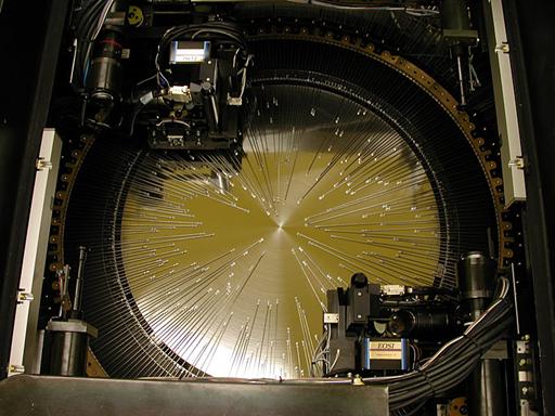
Figure 1. Hectospec focal surface.
2 What
to expect at the Telescope
3 Duties
for Hectospec Observers
4.1 Hectospec ROBOT TV guiders and guide probes
5.1 Initializing the
spectrograph
7 Quick
Look Spectral Extraction
8 Hectospec
Spectrograph Design
8.2 Bench Spectrograph Optical Design
8.2.1 Optical
Design Parameters
8.2.2 Spectrograph
optical Prescription (MM)
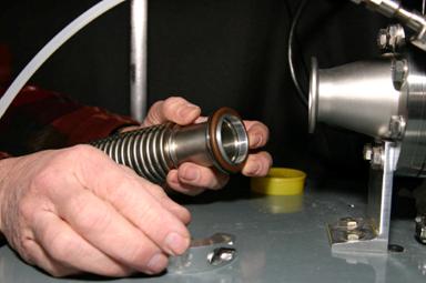
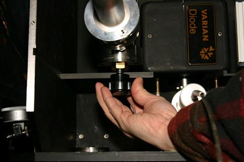
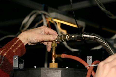
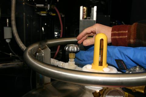
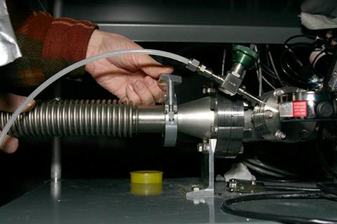
10.1 Pumping
out and Filling the Dewar with LN2
10.2 Bench
Spectrograph & Fiber Reference
10.2.1 Moving Fiber Shoe
Between Hectospec and Hectochelle
10.3 Getting
Bench Ready At beginning of a New run
10.4 Cover
the Optics At the end of the run
11 Hectospec Observing Procedures
11.2.1 Turning on the
Computers in the Control Room
11.2.2 Turning on the
Computers in the f/5 Storage room
11.2.3 Starting up the
software
11.2.4 Turning on the
Power and HOMing the Robots
11.3 Starting
up the Wide Field Corrector
12 Operating the Fiber Positioner
12.1.1 Setting up for
Wavelength Calibration, Domeflats, etc.
12.1.2 Setting up a
configuration for Observation
12.2 Operating
the Bench spectrograph
12.2.3 At the Beginning
of Each night
12.2.4 Starting up the
Calibration lamps
12.4 COmplete
Shutdown
procedure
13 Recovery from Fiber positioner errors
14 Low Level Fiber Positioner Software
14.1 Fiber
Positioner Control software
16.1 Starting
up the WaveFront Sensor
17 APpendix II - Observers cheat sheeT
1 Introduction
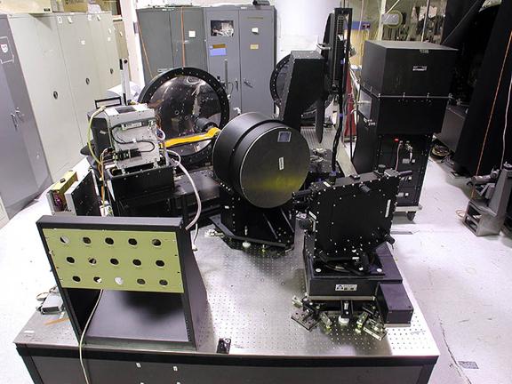
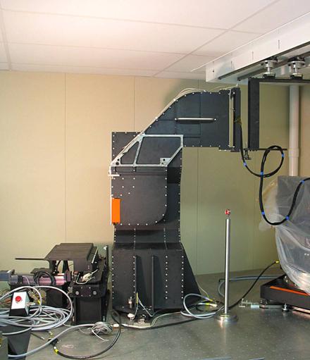
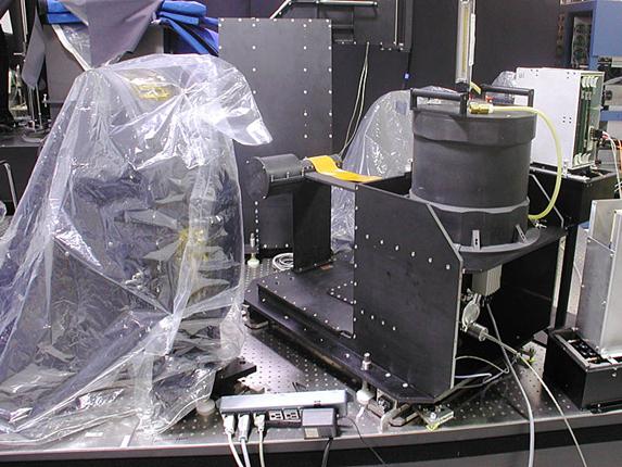
The Hectospec is a multiobject, moderate-dispersion spectrograph that uses a pair of six-axis robots to position 300 optical fiber probes at the f/5 focus of the converted MMT. The converted MMT’s f/5 focus uses a refractive corrector designed by Harland Epps to provide a 1° diameter field optimized for fiber-fed spectroscopy. The Hectospec consists of three major parts: (1) the fiber positioning unit that is mounted on the telescope, (2) a large stationary spectrograph mounted on a 1.8x3.7 m Invar-surfaced optical bench and (3) a 26 m-long bundle of optical fibers connecting the fiber positioner and spectrograph.
The fiber robots position 300 fibers in 300 s to an accuracy of ~25 µm. Each fiber has a core diameter of 250 µm, subtending 1.5² on the sky. Adjacent fibers can be spaced as closely as 20², but the positioning constraints are complicated due to the tube extending from the fiber button to the edge of the focal surface.
Currently
we possess a 270 line mm-1 grating blazed at ~5000 Å
and a 600
line mm-1 grating blazed at ~6000 Å .The efficiency curves
are shown
in Figures 2 and 3.
The detector array consists of two butted EEV CCDs, each with 2048 (spatial dimension) by 4608 (wavelength dimension) pixels. The gap is parallel to a dispersed spectrum. With the 270 line mm-1 grating the spectral coverage is 5770 Å, with a dispersion of 1.21 Å pixel-1. The image FWHM is slightly less than 5 pixels, or ~6 Å.
The fibers are mounted in two rows; images of even and odd fibers are separated by ~30 pixels (in the wavelength direction) at the detector.
Most of the information in this document is for the benefit of the observing staff and the SAO and MMTO personnel responsible for operating the instrument. The astronomer’s duties are limited to preparing the robot configurations for observing and taking data with the bench spectrograph. MMTO and SAO staff will prepare the spectrograph for observing and will fill the dewar.
2 What to expect at the Telescope
This manual contains a great deal of reference information and the volume of this material may intimidate a new user. In fact, much of the material past Section 6 of the manual is mainly of interest to the SAO/CfA personnel who will operate the fiber positioner and make sure that the spectrograph is in operating order. Perry Berlind or Mike Calkins will normally be present during your observing run (very occasionally another CfA person will substitute) to operate the fiber positioner and to provide advice on operating the spectrograph. The CfA robot operator will fill the dewar once a day. Their decisions on operating the fiber positioner safely are not negotiable, and are based on previous operating experience.
The observer’s main responsibilities are to prepare the fields for observation with the planning software, to take data with the spectrograph, and to help replan observations during the night if conditions require a change. Observers should be familiar with the planning software and the instrument constraints described in the next few sections.
The most common error that we have encountered is poor choice of guide stars, including guide stars that are too faint or that are in fact compact galaxies. We strongly recommend guide stars brighter than R=15.5. Observers should use the preview feature in the XFITFIBS software to eliminate galaxies.
Hectospec will be operated in queue mode. Observers may therefore expect to receive a fraction of the clear observing time during each run equivalent to their fraction of allotted time during that run. We try, if at all possible, to observe some of the officially scheduled observer’s fields during their run. If observers are not prepared with valid configuration and catalog files, observations cannot be made.
Currently Nelson Caldwell is responsible for queue scheduling. Nelson attempts to review the submitted files to see if they are valid.
3 Duties for Hectospec Observers
3
We
believe that the queue observing mode for Hectospec and Hectochelle has
been a
scientific and operational success. The Hecto team and FLWO staff
support
the operation of the queue in three ways: (1) SAO scientists and
engineers have
maintained and serviced the instruments as necessary, (2) Nelson
Caldwell has
scheduled the queue observations, and (3) Perry Berlind and Mike
Calkins
have operated the robots. The nightly scientific supervision is the
responsibility of trained observers from the pool of those with
assigned
Hectospec and Hectochelle time. The nights covered by these
astronomers
We would plan to divide each Hecto run into blocks of ~3 nights which would be managed by one or two observers, drawn from the list of astronomers on the proposals granted time. The nights will not necessarily correspond to the assigned nights on the telescope schedule. We have the freedom to shift the times around for the convenience of observers and the queue. During the assigned nights, the astronomer would attend to the following items, which center around insuring that good quality data are obtained.
Observer
Responsibilities
1.
Run the
spectrograph/CCD acquisition
control software
2.
Annotate the
data logs (now under
automation), with comments on conditions, data quality, problems
encountered,
etc.
3.
Check the
operation of the spectrograph/CCD
at the beginning of the night, and monitor readout noise, spectrograph
focus,
thermal flexure, etc. Normally, the
actual focusing would be done by the robot operators, Perry and Mike,
who would
also fill the CCD dewar.
4.
Be
knowledgeable about the fiber assignment
code "xfitfibs", in particular with regard to the restrictions on
rotator position and guide star selection, to the extent of being able
to run
the program at the telescope should the need arise.
5.
Be
knowledgeable about the normal sequence
of operating the positioner and acquiring fields, so that when problems
with acquiring a field occur, the
robot operators
can be advised as to how to proceed (e.g., moving on to another field
because
of poor guide stars). This would not
include actually operating the positioner; that task would remain in
the capable
hands of trained personnel.
6.
Do quick look
reductions of data as it
appears, checking for overall quality, and in particular insuring that
the
spectra fulfill program goals. E.g., are objects detected at all
(coords ok?),
are objects underexposed or overexposed, etc.
7.
Help make
decisions regarding the queue
during times of marginal weather or seeing, choosing targets from the
nightly
list.
To aid the
on-site astronomers, each group
with Hectospec time will be expected to supply a brief summary of their
data
and calibration requirements.
4 Fitting Fibers to Targets
4.1 Hectospec ROBOT TV guiders and guide probes
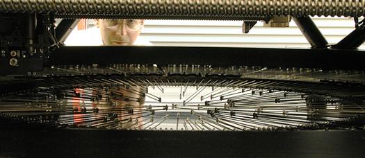
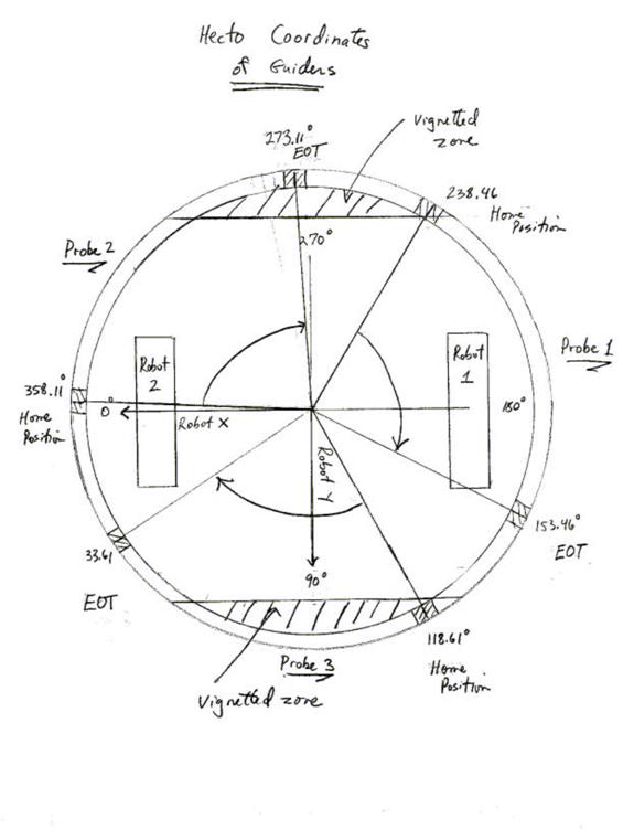
The ease with which the fibers can be initially aligned with respect to the observation targets and the accuracy with which they are kept aligned will affect the overall observing efficiency with Hectospec. Hectospec is guided with at least two guide stars at all times to measure instrument rotator errors as well as telescope altitude and azimuth pointing errors. To avoid occulting prime observing real estate, guiding is performed with three independently actuated probes at the circumference of the focal surface. The probes move along three 86° arcs and each contains relay optics to carry the guide star image to coherent fiber bundles. The three coherent bundles form a trifurcated assembly; the three bundles are brought together to form a single bundle at the input to an intensified CCD guide camera. Because a single guide camera views all of the guide stars, keeping the guide star brightness matched within ~1 magnitude is highly desirable.
In addition, each fiber robot carries an intensified CCD camera that is capable of simultaneously viewing a target object and a backlit fiber through a beam splitter. This
feature was introduced on the Argus multi-object spectrograph at CTIO. After the fibers are positioned for a given observation, the gripper heads will be sent to the intended position of the guide stars and the rotation and pointing errors of the telescope will be removed. The guide stars will then be acquired in the coherent bundles and guiding can begin. If desired, the gripper heads can then be commanded to one or more target objects and the alignment can be checked with reference to a backlit fiber.

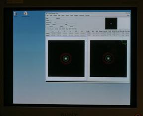
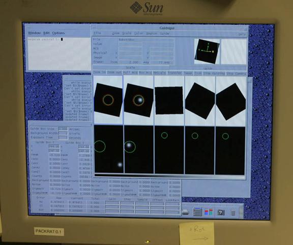
Figure 2. Robot TV guiders that can view the sky and backlit buttons simultaneously.
The guide cameras, manufactured by Electro-Optical Services, Inc., use Gen III image intensifiers with maximum gains of 70,000 and quantum efficiencies of >20% from 4250 to 8750 Å. The camera receiving the trifurcated coherent bundle has its image intensifier photocathode deposited on the back surface of its fiber optic input to avoid defocusing at the photocathode. The image intensifiers are coupled through a reducing fiber optic (1.6:1 ratio for the robot cameras and 2.3:1 for the guide camera) to a 768x493 pixel CCD (each pixel is 11 by 13 µm). The cameras in the fiber positioning robots have a field of view of ~60²x80², while the three coherent bundle guiders each have a field of view of
~30²x 60².
Coherent bundle (one of three) Relay optics
![]()
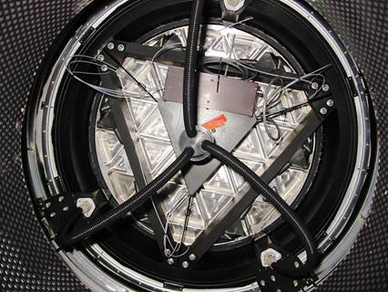
Figure 3.
Photo of trifurcated coherent bundle and guide probes from
beneath the focal surface.
Guide Probe 3 Guide Probe 1 Guide Probe 2 Guide Probe 3 Guide Probe 1 Guide Probe 2![]()
![]()

![]()
![]()
![]()
![]()
![]()
 Figure 4. Position of robots
and guiders with respect to sky when rotator angle is 0°.
Figure 4. Position of robots
and guiders with respect to sky when rotator angle is 0°.
Guide Probe 1 Guide Probe 2
Figure 5. Position
of robots and guide probes in Hectospec specific coordinates.
4.2 Minimizing Rotator Angles
The instrument rotator must track the changing parallactic angle, and the parallactic changes rapidly as a target with a declination near the MMT’s latitude (31.689°) transits.
(The parallactic angle is the angle between two
line
segments originating from the target position, one pointing at the
pole, the
other at the zenith.) We wish to maintain
rotator angles between +/-45° to minimize wear and tear on Hectospec’s
electrical cables and optical fibers. We
have hard limits set near +/-100° but we don’t wish to exercise these
limits. Please plan accordingly by
breaking up
observations into a rising and setting segment if necessary. In any case, the rotator tracking errors
increase to an unacceptable level within about 15-20 minutes of transit
for
targets with declinations within a few degrees of the MMT’s latitude. If your target is north of +50°
declination
or south of +15° declination, you generally do not have to worry about
excessive changes of rotator tracking angles unless your exposure
exceeds 2
hours in length. You do always
need to be sure that guide stars are available for a
rotator angle near 0° at the time of observation regardless of the
declination.
Declination +61.689° +51.689° +41.689° +36.689° +35.689° +34.689° +33.689° +32.689°

Figure 6. The parallactic angle as a function of time in minutes past transit for Northern targets.
Declination +31.689° +30.689° +29.689° +28.689° +27.689° +26.689° +21.689° +11.689° +1.689°

Figure 7. The parallactic angle as a function of time in minutes past transit for Southern targets.
4.3 Running XFITFIBS
4.3.1 Introduction
The PI makes
a catalog of objects, which
may be ranked in preference. The catalog must also include guide stars
on the
same coordinate system. Guiding is done at the edge of the Hectospec
field, not
on the surface where the object fibers are positioned. Thus, there are
very
stringent requirements on guide stars by the small area of sky
available and
the limited range of magnitudes allowed by the TV cameras.
The 2MASS and
GSC II catalogs can be used
where an observer catalog has few stars. In that case, the program tmcguidestars should be used. This
program searches the 2MASS catalog for coincidences with the observer
catalog,
and computes a coordinate transformation. 2MASS and GSC II stars are
selected
in the field, transformed to the observers' catalog coordinate system,
and added
to the catalog. tmcguidestars
is not yet ready for export. It does run on CfA
computers, in a command line mode. External projects should contact
instrument scientists
if they need help with guide star selection.
The PI
downloads the configuration program http://cfa-www.harvard.edu/~john/xfitfibs/
and runs the xfitfibs program for approximate
dates
of observation. In this process, guide
stars are checked for suitability using a number of criteria (magnitude
range,
not a galaxy, no neighbors, etc).
xfitfibs requires
information
such as date and length of observation and number of exposures which
will be used
in scheduling. The output of the program is a number of files which
would now
be sent to a CfA computer for human checking, via the Submit
button.
The
configuration file is modified a few
minutes before the observation takes place, in order to update
positions,
rotation angles, random sky selections, and guide stars.
Please submit
your configuration files at
least 10 days before the run starts.
4.3.2
Brief Instructions
The xfitfibs
program itself contains many pages of help for particular items, and
after
going through these steps, one should consult those pages for detailed
help.
4.3.2.1
Start
by making a catalog.
Starbase
documentation can be
found at:
http://cfa-www.harvard.edu/~john/starbase/starbase.html, but the short story is that this is a tab-delimited ascii format table with a header line:
ra dec object rank type mag
-------------- --------------- --------- ----- --------- ------
2:55:40.217 12:58:42.419 galaxy1 1 target 20.5
2:55:43.304 13:05:04.912 galaxy2 fiducial 15.0
2:55:55.454 13.10:05.234 guide
ra is in hours:min:sec although decimal hours are also okay. dec is in degrees:min:sec although decimal degrees are also okay.
The type column allows the user to insert objects of type fiducial that are used for cross-matching with the 2MASS catalog for guide star selection, but are not assigned to fibers. The default type is target for objects to be assigned to fibers. Type guide is for guide stars.
The object column is optional, but allows the user to name the object.
The rank column gives the target priority; a rank of 1 is highest. Decimal ranks are acceptable.
Additional
columns must have a header, but will be not be used by the subsequent
fiber
assignment software. The input catalog
must have a .stars, .targets, or .gal extension.
It is
essential that the targets and guide
stars be on the same coordinate system.
The
coordinate transformation program is:
http://cfa-www.harvard.edu/jroll/hecto/guidestars-form
You will have difficulty
running the program if the field is dense in stars due to the web
interface
time out limit.
4.3.2.2
Load the catalog and select field centers
4.3.2.2
a. Start up program. this brings up the drawing window and the field window
b. Load a file with pull down menu. This will draw the objects and a 1d circle centered on the objects' centroid, and also make 1 target center in the fld window.
c. In the latter window, enter the start time in UT, e.g.:
March 3
d. Enter an exptime in minutes and nexp (e.g., 15 and 3). (Leave pa, minutes, r0, r1 and r2 alone)
e. For each entry in the field table, enter a priority which will be used in the schedule.
f. If you need sky offsets, please enter those with this format:
#exposures
exptime(minutes)
e.g., 3 2
g. for Chelle observations, select the on-chip binning, either 1x1 or 2x3. Spec projects leave this and the filter blank.
h. for Chelle observations, select the filter. Choices are Ca19, OB21, OB24, OB25, OB26, Na28, RV31, OB32, OB33, OB37, Ca41, iodine, and dumiodine. OB25 is the Halpha filter. See http://cfa-www.harvard.edu/cfa/oir/MMT/MMTI/hectospec/Filter_Specs_a.pdf
i. Click on the box next to the config number (beginning of line), it should turn red indicating it is being operated on.
j. In the drawing window you may now move the circle to where you want it by clicking and dragging, or enter new coords by hand. You may add fields by using the table pull down menu. When you are through moving things around, you should turn those buttons off.
k.
Click on parameters in the
field table
window, and set the # of sky fibers. Once you are happy
with your
field centers, we need to...
4.3.2.3 Select candidate guide stars
4.3.2.3
Click on Fit Guides tab, then begin fit.
The number of
guide stars will appear at
the far right of the fld table row. A red background means too few
stars
available. You may have to move the circle center or change the mag
limit on
the guide stars (at the peril of them not being seen at the telescope).
It may also
be the case that the rotator
angles are red, even though there are enough guide stars.
In this case you can change those angles by
clicking on toggle guide annuli,
going to the drawing window clicking on the (faint) red circle at the
ends of
any of the 3 annuli and dragging the annuli around until r0, r1 and r3
are
green.
Next you need
to classify the guide stars
to remove double stars, stars that are too faint, and plain old
galaxies. Click on classify
candidate. After a while a message
will come back with the results. Some stars may be rejected. Click on ok to rerun the guide star selection.
You can view
the guide stars by bringing up
the Guide window. Use view to select
each configuration in
turn. Clicking on show
will start up ds9 and display all the guide stars in different
frames. Nixed stars may also be seen by using view.
If you are left with no guide stars, you may
try to lower the faint magnitude limit in the parameters menu, but
please
advise us that you have done so, and expect some trouble at the
telescope.
4.3.2.4
Fit Fibers
4.3.2.4
Click on fit fibers, select rank, make depth=7 and begin fit.
Note that all
the field centers you have
entered in the fld table are fit at once, such that no target is
assigned more
than once. If you create two different
output files from the same catalog, by running xfitfibs
at different times with different field centers, then you
may
have
duplicates.
Check to see
that you have fit the number
of targets you expected, otherwise, change your sky fiber numbers in
parameters. Ranking may be changed by
using the rank window.
4.3.2.5 Submit
4.3.2.5
Now you ready
to submit. Click on the Send
tab. Pick the current
trimester (e.g., 2005a),
pick the PI
number, click send. You may get a warning about changed
parameters in the field table, which can be ignored.
A number of files are then sent to CfA, where
they are checked again before being sent out to
Send will
fail if
you did not classify the guide stars. Go back and classify them, and
then run
Fit fibers again.
Send will fail if you did not enter a valid filter or binning for
Chelle
observations. Correct those.
Questions
should be addressed to John Roll john@cfa.harvard.edu or Nelson
Caldwell caldwell@cfa.harvard.edu
5 Taking Data with SPICE
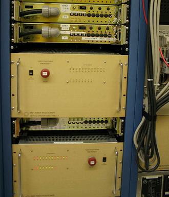
5.1 Initializing the spectrograph
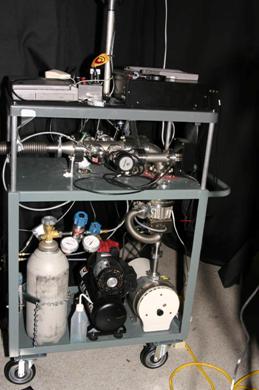
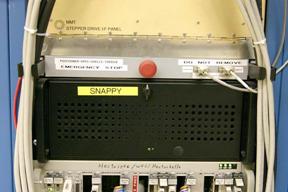
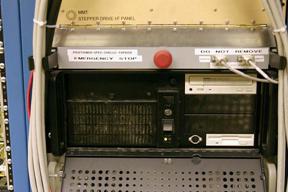
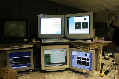
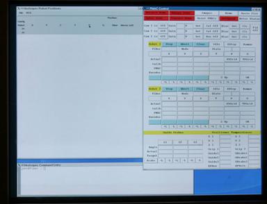
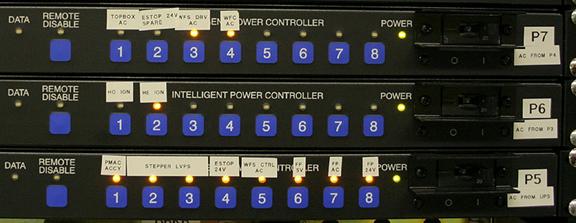
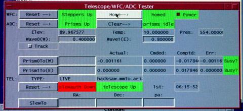
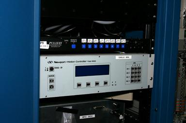
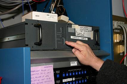
The Hectospec bench spectrograph has 3 motors that need to be powered up and initialized at the beginning of a run, and often at the beginning of each night as well, if power has been shut off for safety. These motors control the CCD dewar focus stage, the grating angle, and the High Speed Shutter (mounted on the fiber shoe). The CCD electronics control and the dome calibration lamps must also be powered up and initialized.
A
suite of three Linux boxes operate the robot positioner, the bench
spectrograph, and the CCD camera (several other computers do work as
well, but
will remain nameless here). The instrument rack on the 2nd
floor must be powered up as described above.
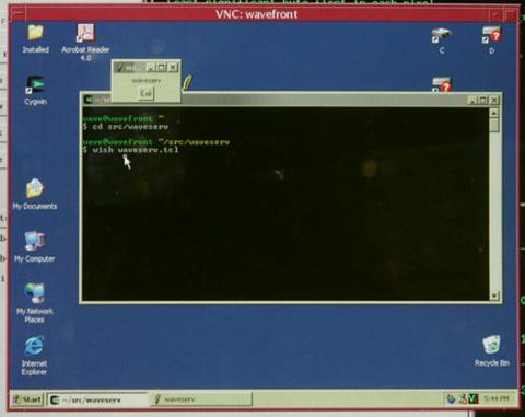
- Login to lewis as spec or chelle as the
case may be. At the beginning
of the run, the robot operator must login to clark and hudson as
well. One keyboard talks to both clark and hudson
- a KVM switch selects which of these is connected to
the keyboard. The switch is a small box and is
usually located near the clark monitors. Login to either clark or
hudson, toggle the switch, and login to the other.
- Open up a shell window
on lewis and type: go.go
- A window called
spicespec or spicechelle should appear, as well as the comment
editor and ds9.
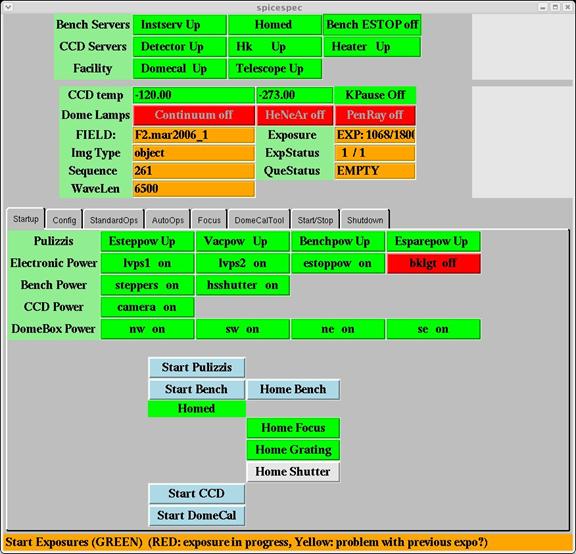
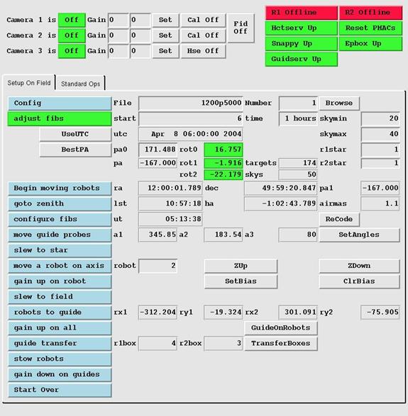
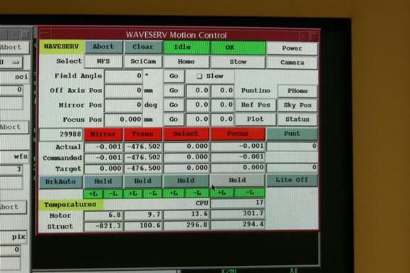
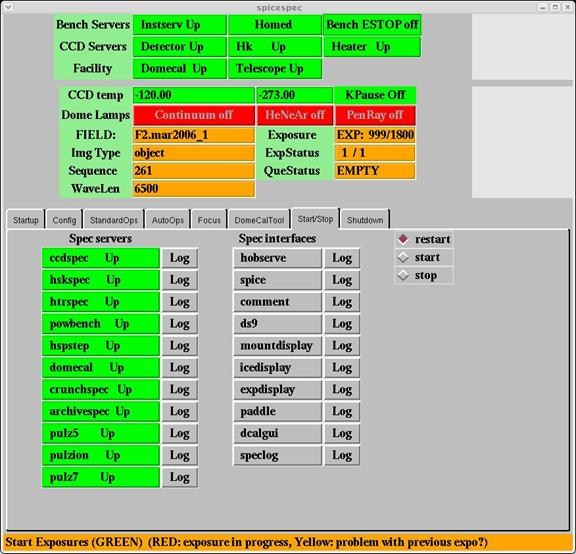
Figure 8. Spice Startup page. Use this to initialize software and home the three spectrograph motors. After this process is complete, return to the startup page for observing.
There
are several tabs in this menu, which can be selected as needed. Initially of course, select “Startup,” which is used to initialize the
spectrograph. The sequence
is: Start Pulizzis,
Start Bench, Home Bench, Start CCD.
The CCD temperature is controlled via a heater in the CCD dewar. If the CCD electronics have been off for a while, say since the previous morning, the temperature will be colder than nominal (perhaps as low as -135 °C) and thus the heater will come on for an extended period till the temperature reaches -120 °C. Thus, for critical measurements, you may wish to monitor this temperature until it reaches nominal, as shown on the Spice upper panel.
The
next tab allows configuration of the bench, e.g., changing the grating
or
grating tilt. Press "ConfigBench" at the begining of the
Hectospec run, or if you have changed either the grating or operating
wavelength. Also on this page, enter the observers’ name. The
Program ID
("Propid") and the PI values will be entered automatically when a
configuration is selected by the robot operator. For testing
purposes,
the telname may be set to "Test", the instrname may be
set to "test", or the detname may be set to "test"
or "specn". Nomally, these should be set to
"mmt_f5_adc", "hectospec" (or "hectochelle"), and
"specs". If the telescope is off however, and you want to take
some test data (darks for instance), then set the telname to "test",
lest an error occur.
The grating, binning and/or the wavelength setting is chosen in this
tab as
well, with only the allowed choices being available in the pull down
menu. 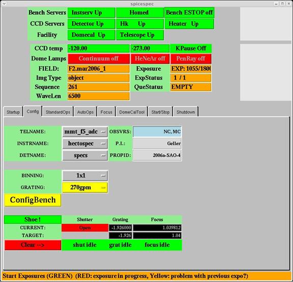
The “Standard Ops” page provides exposure control for the CCD, as well as limited control of the spectrograph and the dome lamps. The control is based on the ICE system.

Figure 9. Spice Standard Ops page for taking spectra. If the box on the lower left above the Pause button is selected, a pull down menu of observation types appears to select the exposure type.
An
exposure is taken by selecting a type of exposure from the pull-down
menu
(shown as obect1 here). Choices include “object”, “comp”
etc. The
number of exposures and the exposure time are taken from the columns to
the
right Go box (green before an exposure, red during an exposure
as shown
here). Click on Go to start an exposure. The user is
prompted for a
title. The Exposure box and queue status shows the
progress. Upon
readout completion, a beep is issued and the file is automatically
displayed
into a ds9 window (called “ds9spec”). To stop an exposure, first pause
it.
File names
will have the naming convention of TYPE.nnnn.fits, where
TYPE is
the fiber configuration name for OBJECT exposures (see above) or the
type of
exposure for all others, and nnnn is a running count number among all
types
of frames. The files are stored in directories created
automatically for each night, with the form:
SPEC/year.monthday.
E.G., SPEC/2004.0409 (If Hectochelle is in use, CHELLE
replaces
SPEC.
The rest of the tabs are described below.
5.2 Kinds of ExposureS
OBJECT: prompts for a title, opens the shutter, writes “object” as imagetype in the header.
SKYOBJECT: prompts for a title, opens the shutter, writes “skyobject” as imagetype in the header. Used for blank sky fields taken between object fields.
SKYFLAT: prompts for a title, opens the shutter, writes “skyflat” as imagetype in the header. Use this for twilight sky exposures.
COMP: prompts for a title, opens the shutter, writes “comp” as imagetype in the header. Use this for dome exposures of HeNeAr etc. Startup the dome lights with the appropriate button for HeNeAr, exposure times of about 5x300 seconds are recommended, multiple exposures are useful to eliminate cosmic rays. With the PenRay HgNeAr combination, shorter exposure times may be used (30 seconds or so).
DOMEFLAT: prompts for a title, opens the shutter, writes “domeflat” as imagetype in the header. Turn on the dome continuum lamps. For the dome continuum exposures with hectospec, an exposure time of 2 seconds is recommended. Shorter exposures may suffer from shutter vignetting, and thus would not be useful for throughput corrections, though the files should still be ok for pixel-pixel flattening.
QFOCUS: Enter the number of exposures desired, the center focus value, and the focus step between exposures. Good values for those are 7, 4, and -0.04. This routine will take a sequence of exposures, at the requested sequence of focus values for the spectrograph, which can then be analyzed. Typically, one uses the dome calibration PenRay lamps for this purpose, though night sky emission lines work well also. The exposure can also be done while the mirror is covered. This program uses the grating in zero order, and the charge is moved between the exposures, thus only one file is produced. The image will have one spot per fiber, per exposure. So the image will have 300 rows of n spots, where n is the number of exposures. Bearing in mind that the in-focus images are not Gaussian but rather flat-topped, a script has been written that analyzes the data frame and produces a plot. In an iraf window, type this command: qfocus filename. A plot in gv will be produced showing image concentration as a function of focus position. Different fibers are shown as different symbols. Higher concentrations are better. Once you have determined the focus, you still must set it using the Focus tab.
FOCUS: Enter the number of exposures desired, the starting focus value, and the focus step between exposures. This routine will take a sequence of frames, at the requested sequence of focus values for the spectrograph. Typically, one uses the dome calibration HeNeAr lamps for this purpose, though night sky emission lines work well also. The focus step size should be about 0.04. Exposure times of the dome HeNeAr should be about 180 sec or longer. Currently, there is no automated routine to choose the best focus, so inspection of the images via iraf imexamine should be used. Bear in mind however, that the in focus images are not Gaussian; rather they are somewhat flat-topped with steep wings (example below). Using imexam “r” will show a profile of emission lines – look for a flat top and a clean, not noisy profile. The FWHM of these profiles should be less than 5 pixels. The focus is the same at all wavelengths and all fibers, though the profiles vary with wavelength (going from FWHM 4.1 in the red to 4.8 in the blue). There is also a slight difference in the PSF in the two CCDs, though the difference is only about 0.2 pixels in width. Recall that the dispersion is about 1.2 Å pixel-1 for the 270 gpm grating.
DARK: prompts for a title, does not open the shutter, writes “dark” as imagetype in the header. There are light leaks around the shutter, so darks should be taken with the chamber lights off. The dark rate is extremely low, and in normal circumstances does not need to be measured. Be aware that the fluorescent lights in the spectrograph room will elevate the dark count significantly for about an hour after they are turned off.
BIAS: prompts for a title, leaves shutter closed, writes “zero” as imagetype in the header. There is some structure to the bias, so we recommend taking a handful of these at the beginning of the night.
5.3 SPICE DETAILS
The autoops tab is not
described here.
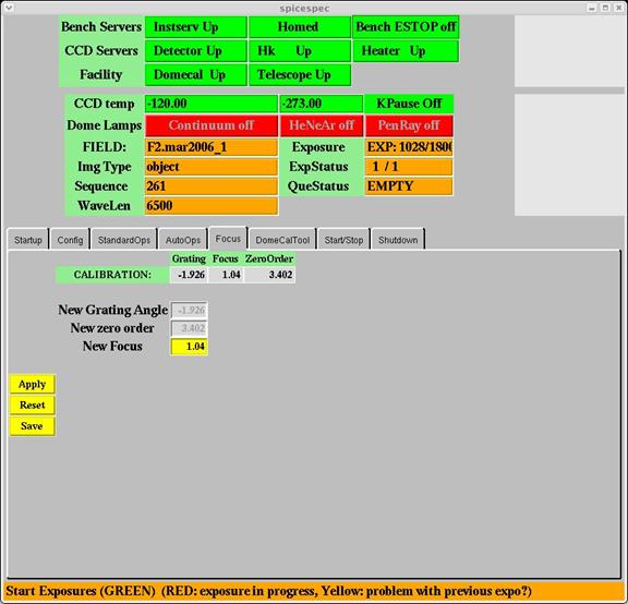
The focus tab is used after determining a new focus. Enter the
correct
value next to new focus, click on apply and set.
The next tab shows the calibration
lamp
status. The lamps themselves are usually controlled in the
standard ops
tab, but this tab shows the details of eack kind of lamp.

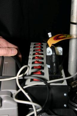
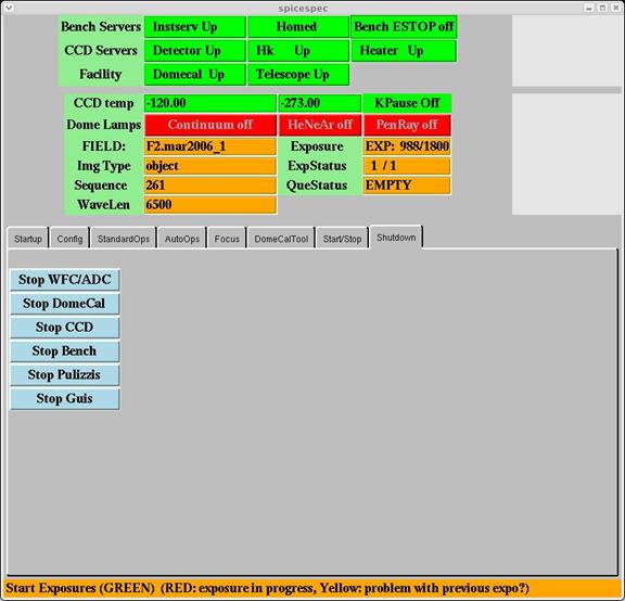
The start/stop tab allows control of the many software servers in the system. Select the action wanted at the middle right ("restart, start, stop"), then click on the button desired to the left (e.g., domecal up).
The shutdown page allows one to shut down the spectrograph and wide field corrector. Normally done by the robot operators.
5.4 Data Logging
The
comment window is used to create and maintain the data logs,
which are
mostly automatic. The one thing the observer can add is a comment
when
needed. In particular, it useful to comment on the seeing and
cloud
presence during the night, and any problems with particular files. To
do so,
first insure that the correct data has been selected (recall that we
use the UT
date). To comment on an existing file, click on its name in the right
panel.
The basic information will appear to the right, and you can now type
into the
comments panel. Click on Save Changes. To edit
an
ongoing exposure, click on Open Current and then enter
comments.
To view the data logs, click on the sunburst button at the bottom
right. A
postscript file is created and the displayed using gv.
Exit gv
using q.

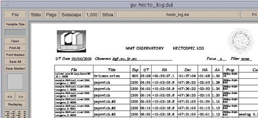
Figure 12 Example data log.
5.5 Data forMat
The A/D converter is 16 bit, so saturation occurs at 65536. There are 2 amplifiers per CCD, and thus the data are stored in FITS extension format, with 5 extensions (0 being the main file header). Among other things, this means that in iraf, you will occasionally have to refer to the file as filename[1] or [2], say when using imheader (though not imexamine).
The data from the different amplifiers are not flipped to the same orientation before writing to disk, but the header keywords allow ds9 to display the files correctly. We hope that all the file keywords are correct, and that programs like IRAF’s mscred will work, but we can’t guarantee this at this time. The SAO version of NOAO’s mscdb package must be installed to use mscred.
As already written, the data files are stored in
directories
of the format /SPEC/ year.monthday (or
CHELLE/ year.monthday . The files are
also archived both on the packrat computer as well as back in
The fiber mapping files (“filename_map”) are stored along with the data files. This information is also stored in the FITS file.
5.6 DS9 BASICS
Each new file is automatically displayed into the active frame of ds9 (named spec9 here to avoid conflicts with other ds9 programs that may be running). To load files off the disk, select FILE:OPEN OTHER: OPEN MOSAIC IRAF, and then find your directory and filename. You may load files into different frames via creating a new frame: FRAME:NEW. Run through frames via Tab. Do not use mscdisplay in IRAF.
The contrast can be changed with the right mouse button. For further contrast levels, select Scale:Scale Parameters from the top bar menu. You’ll get a histogram of the data – high and low values may be selected by moving the red and green vertical lines with the mouse.
Note that the files are shown with blue on the left, thus requiring the XY coordinate system to be non-standard. Image coordinates refer to individual extensions (one per amplifier), and thus start over when crossing into an new extension, while the detector coordinates refer to the combined image. The default display also excludes the overscan areas. To see these, select SCALE and turn off DATASEC. However, some of the overscans will display over that from the next image extension…
Imexamine works as is with these files; there is no need to use mscexamine. Make sure you start up IRAFin a xgterm window.
6 Data Reduction
The data obtained by CfA PIs will be reduced by the Telescope Data Center (TDC) unless the spectrograph operation mode is inconsistent with the standard pipeline or unless the PI wishes to reduce his or her data. For non-CfA users the TDC will make the pipeline software available. Check the TDC website (http://tdc-www.harvard.edu/ ) to download this software. Doug Mink (dmink@cfa.harvard.edu) may be able to provide advice about this software in case of difficulty. Nelson Caldwell is very familiar with the operation and characteristics of the spectrograph, and has a good deal of experience with data reduction. He is willing to provide a limited amount of help to users; he may be contacted at ncaldwell@cfa.harvard.edu.
All Hectospec or Hectochelle data will be archived nightly by the TDC.
7 Quick Look Spectral Extraction
7
A fairly fast
method of extracting all 300
fiber spectra from Hectospec images is provided by a command that runs
a series
of PERL and IRAF scripts. The input is a series of raw images, which
are
processed as described in this document
<http://cfa-www.harvard.edu/oir/MMT/MMTI/hectospec/hecto-reductions.htm>.
The calibration files used are stored in a subdirectory, and may need
to be
remade for every observing run (but not every night). The output is a
FITS file
containing wavelength calibrated, sky-subtracted spectra in multispec
format.
The
program currently runs on lewis.
Here
is what you need to do:
1. Open an xgterm , with xgterm
&. You may resize the font via
shift-middle mouse
button. Start up IRAF with cl.
2.
You'll
need to know the names of the files you want to combine. The IRAF
command
ldata will list the files in the current data directory, or you
can look
at the data logs. The output files will be written in
the
current directory.
3.
For
multiple files, the program detects the cosmic rays by comparing
images,
and interpolates across them in individual frames, The frames are
then
averaged together before extraction begins. For a single
exposure,
the cosmic rays will not be deleted.
4.
In
the IRAF window, you would type :
qspec
file1,file2,file3 [skyfile]
where the files are
of the form listed from the data command, e.g.,
halostar9:30pm_1.1121.fits. The .fits extension
is
unnecessary. The files must be separated by commas with no spaces. The
optional
skyfile would be used when there are sky fibers in the data that are
marked as
objects (“sky-objects”). The format of this file is simply a list with
one
sky-object aperture per line.
5.
The
program takes 1-3 minutes. The files used in the process are then
listed,
along with the names of the output files. If the output file existed
already,
the program will prompt for deletion.
6.
To look at the
spectra, use splot (you may
need to load imred and then specred first, though they are supposed to
be
loaded automatically). To run through the spectra one by one, use the (
and ) keys. The X and Y scales have
been fixed to display low signal spectra well; to scale to the entire
range of
the spectum, type w and then a while viewing a
spectrum. To
smooth, type s.
7. At the
beginning of each Hectospec run, and certainly if the fiber shoe has
been moved from Chelle to Spec, a
crude wavelength adjustment must be made.
Inspect the exracted spectra which have not been skysubtracted
from any
of your images. Using splot, determine
the wavelength of the brightest night sky line whose wavelength is
supposed to
be 5577A (but which may be off a little because of the problem we are
about to
fix). Subtract the measured wavelength
from 5577 (i.e., 5577-wave_observed). In Spice, select the
configure
tab, and locate the quick look wavelength offset window. Enter the
wavelength
offset in this window and click on save.
Now rerun the extraction. The skysubtraction should work
properly now.
Trouble
may ensue if there are no sky fibers in apertures 1-150 or 151-300.
A
ds9 regions file can be brought up to identify all the apertures and
which
fibers they correspond to. Click on regions, and load regions, and
select the
file /h/spec/specaps.reg.
8 Hectospec Spectrograph Design
8.1 Introduction
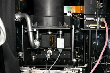
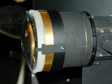
The optics of the bench spectrograph are quite simple. A spherical collimator mirror operating at f/5.4 is used because the imaging is independent of field angle if the fibers are arranged so as to point at the local normal to the mirror. At f/5 the spherical aberration is negligible. The camera is also a reflective system with a spherical mirror and two all-spherical silica corrector lenses and a silica field flattener lens that serves as the dewar window. The camera is based on the Keck HIRES camera, and was designed by Harland Epps.
Collimator Mirror
Optical Fibers Grating
Focus Camera
Mirror![]()

![]()
![]()
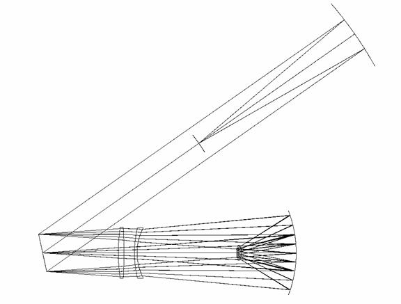
Figure 14. Optical layout of the bench spectrograph. The fibers are arranged in a line perpendicular to the plane of the page.
8.2 Bench Spectrograph Optical Design
8.2.1 Optical Design Parameters
|
Collimated beam diameter |
259 mm |
|
Camera focal length |
397 mm |
|
Fiber core/cladding/buffer |
250/275/300 µm |
|
Fiber subtends on the sky |
1.5² |
|
Reduction (spatial) |
3.45 |
|
CCD format (max) |
4608x4096 pixels |
|
CCD format (nominal) |
3400x3400 pixels |
|
CCD pixel size |
13.5 µm |
|
250 µm fiber sampling |
5.4 pixels |
|
Max. monochromatic beam to camera |
259x344 mm |
|
Camera field radius |
4.7° |
|
Camera-collimator angle |
35° |
|
Camera-grating distance |
546 mm |
|
Camera entrance aperture |
411 mm |
8.2.1.1
8.2.2 Spectrograph optical Prescription (MM)
File : C:\docs\Zemax_Files\hecto\R815_270_as_built_thk.ZMX
Title: HECTOSPEC, RUN 815,
Date :
Surf Type Radius Thickness Glass Diameter Conic
OBJ STANDARD -1375.105 -1371.600 148.345 0
STO STANDARD Infinity 1371.600 254.000 0
2 STANDARD -1375.105 1373.060 148.350 0
3 STANDARD -2748.153 -2748.788 MIRROR 548.278 0
4 COORDBRK - 0 - -
5 DGRATING Infinity 0 MIRROR 275.647 0
6 COORDBRK - 546.100 - -
7 STANDARD 1247.082 40.749 SIL5C 364.794 0
8 STANDARD -3195.945 75.446 365.375 0
9 STANDARD 748.157 19.164 SIL5C 363.988 0
10 STANDARD 387.373 1147.005 357.365 0
11 STANDARD -844.093 -394.829 MIRROR 605.782 0
12 STANDARD -102.083 -25.105 SIL5C 106.132 0
13 STANDARD -582.981 -9.446 90.059 0
IMA STANDARD Infinity 71.338 0
For a central wavelength
of 6563 Å:
Coordinate Break Surface 4: Tilt About X : 22.83°
Diffraction Grating Surface 5: Lines / Micron : 0.27
Coordinate Break Surface 6: Tilt About X : 12.17°
8.3 Grating Choices
The initial grating is a 270 groove/mm grating blazed at 5200 Å purchased from David Richardson Grating Laboratory. The spectral coverage, spectral resolution, anamorphic magnification, grating angles and RMS image diameters with this grating and two possible higher dispersion gratings, all set up with Ha as the central wavelength, are shown below. The spectral coverages in this table refer to the nominal 3400 pixel format. However, the image quality holds up quite well over the whole 4608 pixel format, and the full spectral coverage is ~1.35 times that shown in the table. Remember that second order contamination may be an issue for some applications. Currently, we do not have order blocking filters, but they could be installed.
|
Ruling Density (gpm) |
Spectral Coverage (Å) |
Spectral Resolution (Å) |
Anamorph. Mag. |
Angle of Incidence |
Angle of Diffraction |
RMS Image Diameter (pixels) |
|
270 |
4488-8664 |
6.2 |
1.06 |
22.83 |
12.17 |
1.3-1.8 |
|
600 |
5609-7522 |
2.6 |
1.14 |
29.41 |
5.59 |
1.3-1.8 |
|
1200 |
6084-7038 |
1.1 |
1.33 |
41.89 |
-6.89 |
1.4-1.7 |
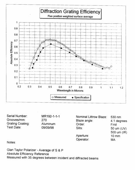
Figure 15. The efficiency of the 270 line grating

Figure 16. The efficiency of the 600 line grating.
9 Spectrograph Performance
9.1 Calculated Throughput
The Hectospec optical layout is simple enough that very high throughput can be achieved if good reflective coatings are used on the mirrors (2 surfaces) and good antireflection coatings are used on the lenses (6 fused silica surfaces). We have used the same dielectrically-enhanced silver reflective coatings and Sol-gel antireflection coatings that we used in the efficient FAST spectrograph. Our predictions for Hectospec's overall throughput with the 270 line grating are shown below. The column labeled “Add. Fiber Losses” includes FRD, end reflection losses, and the losses from misalignments of the fiber axis with respect to the chief ray at the f/5 focal surface. This table does not include aperture losses at the fiber input, which will depend on the seeing and the quality of the astrometry of the targets and the guide stars.
|
Wave |
Mirror Refl. (2 surf) |
Lens Thrput (6 surf) |
Fiber Thrput (26 m) |
Add. Fiber Losses |
CCD Effic. |
|
Grat Effic. |
Tele Refl + 10 cor surf) |
Final Throughput, Hectospec plus Telescope Optics |
|
3650 |
0.90 |
0.89 |
0.70 |
0.80 |
0.66 |
0.80 |
0.37 |
.66 |
0.06 |
|
4000 |
0.90 |
0.92 |
0.80 |
0.80 |
0.80 |
0.80 |
0.49 |
.70 |
0.12 |
|
5000 |
0.91 |
0.98 |
0.90 |
0.80 |
0.85 |
0.80 |
0.66 |
.79 |
0.23 |
|
6000 |
0.92 |
0.98 |
0.94 |
0.80 |
0.80 |
0.80 |
0.61 |
.79 |
0.21 |
|
7000 |
0.92 |
0.98 |
0.96 |
0.80 |
0.75 |
0.80 |
0.53 |
.75 |
0.17 |
|
8000 |
0.92 |
0.95 |
0.98 |
0.80 |
0.60 |
0.80 |
0.43 |
.66 |
0.09 |
|
9000 |
0.92 |
0.91 |
0.98 |
0.80 |
0.30 |
0.80 |
0.37 |
.65 |
0.04 |
9.2 Measured Performance
We can compare the throughput predictions with measurements of a spectrophotometric flux standard star BD+284211 in 1″ seeing. BD+284211 was stepped across a fiber entrance aperture to find the position where we detected the maximum flux.
For an apples to apples comparison we need to correct the measurement for the aperture loss.


Figure 17. Measured throughput in 1″ seeing not corrected for aperture losses.
The appropriate aperture correction for the plots above (measured with Megacam images) is about 1.7 (ratio of flux within a 20″ diameter aperture to the flux within a 1.5″ diameter aperture). Therefore, the peak throughput for light that hits the fiber aperture is about 17% (to be compared with the prediction of 23%) . If we average over wavelength, the measured throughput is about 75% to 80% of the predicted numbers.
We present two “real-world” performance plots: the SNR pixel-1 for a 15 minute exposure as a function of aperture magnitude and the absorption line SNR (1+R) for 45 minutes of exposure as a function of aperture magnitude.
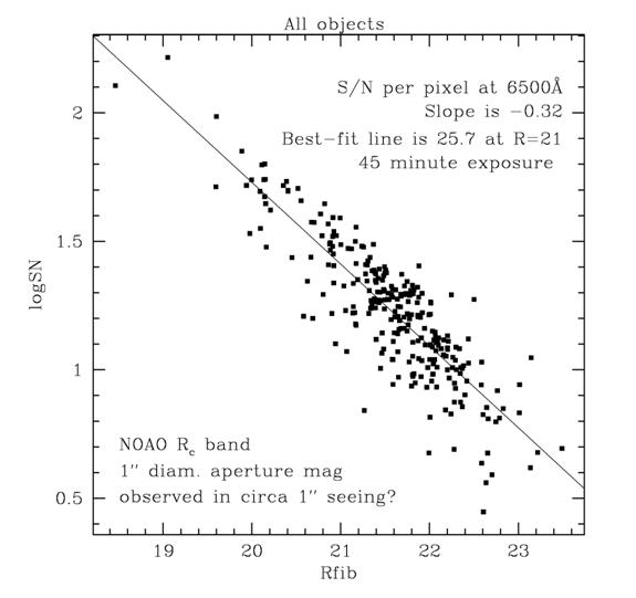
Figure 18. The signal-to-noise ratio per pixel for a 45 minute exposure as a function of aperture magnitude (1² diameter aperture.) The SNR per pixel is ~26 at R=21. The relations for 4500 Å and 8500 Å have the similar slopes, but show a SNR per pixel of ~9 at an aperture magnitude of R=21 for the same exposure length. Improvements in sky subtraction techniques may allow improvement at 8500 Å . Analysis and plot courtesy of Daniel Eisenstein.

Figure 19. The absorption line cross-correlation signal-to-noise ratio (~1+R) for 45 minutes of exposure as function of R aperture magnitude (2.6² diameter aperture). All of the 1974 galaxies in this plot had reliable redshifts. The SNR ratio shown here is reduced somewhat by the use of templates from the FAST spectrograph. Better cross-correlation templates will be created. Courtesy of Michael Kurtz.